An attempt at modelling of cutting forces in oak peripheral milling

Abstract

An attempt was made to evaluate the non-linear, multi-variable dependency between the main (tangential) force, FC, and machining parameters and properties of pedunculate oak (Quercus robur) during straight edge, peripheral milling. The tangential force, FC, was found to be influenced by the feed rate per tooth, fZ, cutting depth, cD, rake angle γF, Brinell hardness, H, bending strength, RB, and modulus of longitudinal elasticity, E. Several interactions between machining parameters and properties of wood were confirmed in the developed relationship FC = f(fZ, cD, γF, H, RB, E).

Full Article

An Attempt at Modelling of Cutting Forces in Oak Peripheral Milling

Marija Mandić,^a Bolesław Porankiewicz,^b,* and Gradimir Danon ^a

This paper presents an attempt at the evaluation of the non-linear, multi variable dependency between the main (tangential) force, F_C, and the machining parameters and properties of Pedunculate oak (Quercus robur) during, straight edge, peripheral milling. Tangential force, F_C, was found to be influenced by density, D, moisture content, m_C,  Brinell hardness, H, bending strength, R_B, the modulus of elasticity, E, feed rate per tooth, f_Z, rake angle, γ_F, and cutting depth, c_D. Several interactions between the machining parameters and properties of wood were confirmed in the developed relationship F_C= f(D, m_C, H, R_B, E, f_Z, c_D, γ_F,).

Keywords: Oak; Properties of wood; Machining parameters; Peripheral milling; Main cutting force

Contact information: a: Department of Wood Processing, University of Belgrade- Faculty of Forestry, Belgrade, Serbia; b: Poznań University of Technology, Poland;

* Corresponding author: poranek@amu.edu.pl

INTRODUCTION

The contemporary theory of wood machining seems to have been developed on the basis of the metal processing theory (Afanasev 1961; Beršadskij 1967; Glebov 2007; Manžos 1974; Amalitskij and Lûbčenko 1977). An attempt to base the wood cutting theory on the mechanical properties of wood for three main and intermediate cutting directions (modes) has already been made (Deševoy 1939). Factors with an impact on the mechanics of wood cutting (and chip formation) can be divided into three groups (Eyma et al. 2004; Naylor and Hackney 2013): wood species, wood properties, and the cutting process itself. The research by Franz (1958) was aimed at the main and normal cutting force analysis (with the use of a dynamometer equipped with an electrical resistance strain-gage bridge and strain-analyzing instrument). Several mechanical properties, including tensile strength perpendicular to grain, R_T⊥, modulus of elasticity in tensile parallel to grain, E, modulus of rupture in bending, R_B, modulus of elasticity in bending, E_B, crushing strength parallel to grain, R_C॥, shear strength parallel to grain, R_S॥, and cleavage, R_CL, were evaluated for moisture contents of 3%, 11%, and 30%, using wood specimens of yellow birch (Betula alleghaniensis Britt.), sugar pine (Pinus lambertiana Dougl.) and white ash (Fraxinus americana L.).

Various research articles (Kivimaa 1950; Franz 1958; McKenzie 1960; Koch 1964; Woodson and Koch 1970; Axelsson et al. 1993; McKenzie et al. 1999) have discussed the impacts of the stated factors on cutting forces and chip formation, the durability of tools, the precision of processing and the quality of processed surfaces. The primary objective of these studies was to better understand the interaction between a tool and processed item for the purpose of a more efficient management of the cutting processes. In addition, energy and tool saving methods are also important. However, in this case, they stay in the background.

The literature dealing with mechanical wood processing reveals various methods for anticipating/calculating cutting forces. In many approaches, these are coefficient methods, in which authors start from the referent unit cutting resistance for a certain wood species, most frequently pine wood, which is calculated under strictly defined and controlled (standard) conditions (Afanasev 1961; Beršadskij 1967; Glebov 2007; Manžos 1974; Amalitskij and Lûbčenko 1977; Orlicz 1982; Goglia 1994). Specific cutting resistances for certain materials and certain cutting conditions (for all possible wood grain orientation angles or cutting modes) are obtained by multiplying referent unit cutting resistances and appropriate correction coefficients, which can be found in adequate tables. Orlicz (1982) pointed out that differences between forces calculated using the coefficient method and forces measured in experiments reached as much as 40%. In certain cases, this difference was more than 100% (Mandić et al. 2014). There are several possible reasons for the discrepancies, but one of the primary reasons is the fact that physical and mechanical properties of wood are not sufficiently and properly included in the stated models. It is known from the literature that physical and mechanical properties of wood depends on the environmental conditions in which the tree grew up, as well as on the position of the longitudinal and transverse cross-sections of the trunk (Krzysik 1975).

Eyma et al. (2004) would have offered an interesting, novel approach by applying several mechanical properties of wood of 13 species to cutting forces analysis. However, instead of the main (tangential) cutting force, F_C, the resultant cutting force, F_R=(F_C²+F_N²)^0.5 was taken into account in this study, making the study of all cutting forces useless in the opinion of the authors.

Better results in anticipating cutting forces can be achieved by establishing a model that would include both physical and mechanical properties of wood in addition to the cutting regime. These models are usually established based on extensive experiments involving various wood species and cutting conditions. A disadvantage is the fact that tests are most frequently conducted on specially designed equipment and/or at small cutting speeds, thus not providing a sufficient level of generality. The role of the applied measuring equipment in the observed discrepancies should also be taken into consideration (Feomentin 2007).

In practice, wood machining is rarely conducted in pure general cases (modes): perpendicular (⊥), parallel (∥), or transversal (∦). These cutting cases were also examined in the past (Time 1870; Deševoy 1939). In the study by Kivimaa (1950), these cases were first defined as A, B, and C, respectively, and further used in many studies. A more general approach to applying the three wood grain orientation angles towards the cutting edge, φ_K, towards the vector of cutting speed velocity, φ_V, and towards the cutting plane, φ_S, can be found in the research by Orlicz (1982). This approach allows for the analysis of all intermediate cutting cases as well as defining the general case.

Another model, published in the study of Porankiewicz et al. (2011) was produced and verified on the research results of the study Axelsson et al. (1993). The model includes physical properties of the samples, tool characteristics, and characteristics of the processing regime. The study provides statistical equations for tangential, F_C and normal, F_N, cutting forces in the function of wood grain orientation angles (from perpendicular to parallel), edge radius round up, ρ, rake angle, γ_F, mean thickness of a cutting layer (chip thickness), a_P, cutting speed, v_C, wood density, D, and moisture content, m_C, (8% to 133%) and temperature of wood, T, developed from an incomplete experimental matrix.

Another approach (Eqs. 1 through 3) evaluating the relationship F_C= f(g_F, r, a_P, D, m_C, not taking into account wood grain orientation angles and cutting speed, v_C, was published by Ettelt and Gittel (2004), Tröger and Scholz (2005), and Scholz et al. (2009). These solutions were based on the research of Kivimaa (1950) and refer to the defined cutting modes. In the authors’ opinion, it is difficult to find justification for the use of the following equations:

k_C0.5= F_C ⋅ a_P^-1/2 (1)

k_C0.5=f_t ⋅ w_C ⋅ a_P^1/2 (2)

and

f_t= f( ,φ) (3)

where k_C is the specific cutting resistance (N·mm^-1/2), f_t is a linear function, taking into account cutting modes,  is the angle between wood grains and cutting edge, and φ is the angle between the wood grains and the cutting velocity vector.

A linear model, F_C = f(γ_F, ρ, a_P, D, m_C, φ), was recently published for rotary cutting of two African wood species for three basic cutting cases (modes) (⊥- A, ∥ – B and ∦ – C), employing one wood grain orientation angle φ (Cristóvão et al. 2012). Literature surveys show that the dependence of the main cutting force on all cutting parameters, in a wide range of variation, is non-linear, so the choice of linear model in the cited work does not appear to be appropriate. Furthermore, the use of only one wood grain orientation angle φ to define three basic cutting cases (modes) in one linear model, appears to be a fundamental error. Three orientation angles are necessary for precise definition of cutting cases: φ_E – between wood grain and the cutting edge, CE; φ_V – between wood grain and the vector of the cutting velocity, v_C, and φ_C – between the wood grain and the cutting plane (Orlicz 1982; Porankiewicz 2014).

The present study is an attempt at the evaluation of the relationship between the main (tangential) cutting force, F_C, by peripheral oak wood milling and machining parameters: – cutting depth, c_D, and feed per edge, f_Z, rake angle, g_F, as well as the physical properties of wood: – wood density, D, moisture content, m_C, and some mechanical properties: – bending strength, R_B, modulus of elasticity, E, and Brinell hardness, H.  The other parameters: – cutting edge round up radius, r, cutting speed, v_C – the diameter of the cutter, D_C, cutter width, W_C, and the number of cutting edges, z, were kept constant. The present study will also to a certain degree allow verification of the relationship K=f(c_D, f_Z) between relative cutting resistance, K, cutting depth, c_D, and feed rate per edge, f_Z, published in the study by Orlicz (1984) for pine wood and applied on oak wood after the use of the coefficient of wood species c_R=1.55 (1.5 – 1.6).

EXPERIMENTAL

The testing materials included radially cut samples for the determination of physical and mechanical properties of pedunculate oak (Quercus robur).

Physical and mechanical properties were tested in accordance with various standards, i.e. standards for density (SRPS D.A1.044, 1979), bending strength (SRPS D.A1.046, 1979), Brinell hardness perpendicular to wood grains in the radial direction (EN 1534, 2011) and for the modulus of elasticity (SRPS D.A1.046).

Fig. 1. The cutting situation by longitudinal milling with the use of a cutter with a hole; a_P – the average thickness of the cutting layer; y_A – average meeting angle; y₁ – maximum meeting angle; P_F – working plane; P_R – main plane; P_P – back plane

The testing during peripheral wood milling was performed on a table mounted milling machine MiniMax, equipped with a 3 kW three phase asynchronous electrical motor. The accessory motion was achieved using a Maggi Engineering feeding machine Vario Feed, with speeds ranging between 3 and 24 m∙min^-1 and a three phase asynchronous electrical motor with the nominal power of 0.45 kW. The milling cases were up-milling, opened and peripheral milling. Three cutters were used of diameter 125 mm, and a width of 40 mm, equipped with four soldered plates, made of cemented carbide H302 manufactured by Freud, Italy. The edges had a radius of the round up ρ= 2 µm. The roughness of rake and clearance surfaces, after regrinding with grinding wheels D76, D46 and D7 for rough finishing and final finishing were of R_aa = 0.15 mm and R_ag = 0.18 mm, respectively. The cutters had a clearance angle a_F= 15° and three different rake angles, g_F, namely 16°, 20° and 25°.The orientation angle of wood grains towards the cutting edge was j_K= 90°. The average wood grain orientation angle toward the cutting speed velocity vector was in the range j_V<0.1241; 0.1908 rad>, and that toward the cutting plane was in the range j_S<0.1241; 0.1908 rad>.

The testing was performed with a constant RPM of the working spindle, i.e. n= 5,860 RPM, at a constant cutting speed v_C= 38.35 m·s^-1, at three feeding speeds v_F= 4, 8, and 16 m·min^-1 and at cutting depths of wood c_D= 2, 3, and 4.5 mm.

The rotational speed of the tool spindle, n, was measured under load, with the use of a digital, non-contact tachometer, type PCE-DT 65, manufactured by PCE Instruments.

The cutting power was measured indirectly using the power input of the machine driving the electric motor. The measuring device SRD1, connected with a computer, was used for measuring, with a sampling frequency of 1 kHz. The device uses the Power Expert program package developed in cooperation with the Center for Wood Processing Machines and Tools and the Unolux Company from Belgrade. Fig. 2 presents a typical record of the cutting power and the manner of its processing.

Fig. 2. Procedure for processing the results of cutting power measurements during peripheral milling

It can be seen in Fig. 2 that the shape of the record was a rounded trapezium. In the graph, values of total power, P_total, power when idle, P_O, and power required for cutting, P_C, are presented, with the power required for cutting being the difference between the first two values:

P_C= P_total – P_O (W) (4)

Average values of the measured powers, based on a higher number cuts on the same test sample, were used for calculating mean values of the main cutting resistance by using the following Eq. 5,

F_mean= P_cmean · v_C^-1 (N) (5)

where F_mean is the mean value of main cutting force for one revolution of the tool; P_cmean is the average cutting power (W), and v_C is the cutting speed (m·s^-1).

The calculated value of the mean force, F_mean, is the mean force for one rotation of the tool, which means that it also includes idle time between the cutting rotations of the four blades (Fig. 3)

Fig. 3. Tangential cutting forces during one revolution of the cutter; – cutting edge rotation angle; ₁ – maximum edge meeting angle

For obtaining the average main cutting force per one edge, F_C, it is necessary to correct the value of mean force, F_mean, as follows,

F_C =F_mean ⋅ O_gl ⋅ S l_r1^-1 = F_mean ⋅ 2 ⋅ p ⋅ ( i ⋅ y_M )^-1 (N)  (6)

y_M = y₁ + y₂ (rad) (7)

where: O_gl is the circumference of the cutter (m); l_r1 is the length of cutting of one edge (m); i is the number of cutting edges; R_C  is the cutting radius (m), and y_M is the rotation angle of the cutting edges in the object (Fig. 1).

For each of the 22specimens, at least four measurements of physical and mechanical properties were conducted. The measured density, D values were within the range of 613 kg·m^-3 to 790 kg·m^-3. The width of the cut was W_C= 30 mm.

As already mentioned, the testing was conducted for various combinations of cutting process parameters. The peripheral milling process parameters are given in Table 1.

Table 1. Peripheral Milling Process Parameters of Oak

Table 2 shows the derived values of the mean cutting layer thickness (chip thickness), a_p and angle between the cutting velocity vector, v_C and wood grains, j_V.

Table 2. Derived Peripheral Milling Process Parameters of Oak

The measurements were repeated at least eight times for each combination of processing parameters. Based on the calculated average forces, the relationship F_C= f(D, m_C, H, R_B, E, f_Z, γ_F, c_D) was estimated in preliminary calculations for linear, polynomial, and power types of functions, with and without interactions. The model should fit the experimental matrix by the lowest summation of residuals square, S_K, by the lowest standard deviation of residuals, S_R, and by the highest correlation coefficient of predicted and observed values, R. The experimental matrix can be fitted with simpler models, but this will result in a decreased approximation quality, which means that the S_K and S_R values will increase and R will decrease. It must be pointed out that an empirical formula can be valid only for ranges of independent variables chosen within the experimental matrix, especially for incomplete experimental matrices and complicated mathematical formulas with interactions.

In this case, all predicted values of the dependent variable will have a higher expected error. Many years of experience by the authors suggest that efforts to fit such data with overly simple models can be expected to hurt the quality of the approximation, especially in the case of variables with small importance, making such a model nonsensical. Proper influence of low importance variables can be extracted only from an experimental matrix when using a more complicated model. The most adequate formulas appeared to be non-linear multi variable equations with interactions, Eqs. 8 through 11:

F_C^P= A+B+C (8)

where

A= e₁ · D₈^e2 · m_C^e3 · H^e4 · R_B^e5 · E^e6 · f_Z^e7 · γ_F^e8 · c_D^e9 (9)

B= e₁₀ · f_Z · c_D+e₁₁· f_Z · γ_F+e₁₂ · R_B · f_Z+e₁₃ · R_B · γ_F (10)

C=e₁₄ · D₈ · E+e₁₅ · D₈ · f_Z+e₁₆ · m_C · R_B+e₁₇ (11)

Estimators were evaluated from an incomplete experimental matrix having 22 data points. During the evaluation process of the chosen mathematical models, the elimination of unimportant or low important estimators was carried out by use of the coefficient of relative importance, C_RI. The C_RI is defined by Eq. 12 and with the assumption C_RI > 0.1:

C_RI= (S_k+S_RI) · S_k^-1 · 100 (%) (12)

In Eq. 12, the new terms are S_K0k, the summation of square of residuals for estimator a_k = 0. In this equation, a_k is the estimator of the number k in the statistical model evaluated.

Figure 4 shows a flow chart of the optimization program used.

Fig. 4. Flow chart of the optimization program; variants: MC- Monte Carlo, G- gradient, MCG- combined MC and G, S_K– summation of square of residuals, R– correlation coefficient, S_R– standard deviation of residuals

The summation of the square of residuals, S_K, standard deviation of residuals, S_R, correlation coefficient, R, and the square of correlation coefficient between the predicted and observed values, R², were used for the characterization of the approximation quality. The calculation was performed at the Poznań Networking & Supercomputing Centre (PCSS) on an SGI Altix 3700 machine, using an optimization program based on the least squares method combined with the gradient and Monte Carlo methods (Fig. 4).

RESULTS AND DISCUSSION

The final shape of the approximated dependence, Eqs. 8 through 11, using the optimization program shown in Fig. 4, was obtained after 7.54·10⁹  iterations.

The following estimators were evaluated: e₁= 0.68806; e₂= 0.62019; e₃= 0.18212; e₄= 0.045741; e₅= 0.27236; e₆= 0.53737; e₇= 0.54972, e₈= -0.50384; e₉= 106.55693;        e₁₀= -14.2737; e₁₁= -1.80803; e₁₂= -7.0966·10^-3; e₁₃= -7.53491·10^-6; e₁₄= -0.056067;        e₁₅= 0.038487; e₁₆= 0.01174; e₁₇= -14.60027.

The rounding of the estimator values to the 5^th decimal place produced an acceptable deterioration of the fit 0.005%. Reducing the number of the rounded decimal digits to 4, 3, 2 and 1 would cause unacceptable deterioration of the fit as much as 15%, 85%, 96% and 3927%, respectively.

The coefficients of relative importance, C_RI, for the estimators have the following values: C_RI1=159517; C_RI2=816197; C_RI3=404687; C_RI4=63793; C_RI5=1383657; C_RI6=725575; C_RI7=1070522; C_RI8=815139; C_RI9=764929; C_RI10=572373; C_RI11=313681; C_RI12= 9737; C_RI13=127516; C_RI14=10564; C_RI15=36463; C_RI16=1629705; C_RI17=6637.

For each of the 22 combinations of input data, the predicted tangential cutting forces, F_c^p were calculated using Eqs. 8 through 11. These results are shown in Fig. 5. The approximation quality of the fit, also seen in Fig. 5, can be characterized by the quantifiers S_K= 70.94; R= 0.995; R²= 0.991; and S_R= 1.88.

Equations 8 through 11, after substituting estimators from e₁ to e₁₇, take the following forms: 

F_C^P= A+B+C                                                                                                  (13)

where:

A=0.01174·D^0.68806·m_C^0.62019·H^0.18212·R_B^0.045741·E^0.27236·f_Z^0.53737·γ_F^0.54972·c_D^-0.50384       (14)

B=106.55693·f_Z·c_D – 14.2737·f_Z·γ_F – 1.80803·R_b·f_Z – 7.0966·10^-3 · R_B·γ_F                     (15)     

C=-7.53491·10^-6· D ·E – 0.056067 · D · f_Z + 0.038487 · R_B  -14.60027                     (16)

Fig. 5 shows that the maximum deviation from Eqs.13 through 16 was as high as S_R= 5.27 N. For the minimum and maximum values of the F_C, the points lay closer to the regression straight line. These equations provide a strong link between the observed and predicted cutting forces and can be used to analyze the impact of specific inputs on the predicted cutting forces.

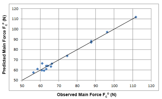
Fig. 5. The plot of the observed main force F_C^O against the predicted F_C^P values, according to Eqs. 13 through 16

Figure 6 shows a plot of the relationships among the main cutting force, F_c^P, the cutting depth, c_D, and the rake angle, γ_F. Figure 6 shows that F_C^P strongly, non-linearly  depends on c_D in a parabolic decreasing manner. An increase in c_D increased F_C^P, more for a lower γ_F. The average change of F_C^P with an increase in the cutting depth, c_D, by 0.1 mm is between 4 N and 2.6 N, depending on the size of the rake angle, γ_F. An increase in γ_F increases F_C^P for the largest cutting depth, c_D. As c_D fell below ~3 mm, a minimum started to appear. For the lowest c_D, the influence of γ_F on F_C^P was small, with a minimum at γ_F ~21.4° at c_D = 2.5 mm. The relationship F_C^P = f(c_D) combines the influence of increasing cutting layer thickness (chip thickness), a_p,  and to a lesser degree the influence of increasing grain orientation angle, φ_V.

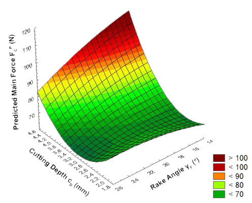
Fig. 6. The plot of the relationships among the predicted main force F_C^P (N), g_F (^o), and c_D (mm), according to Eqs. 13 through 16; D= 750 kg·m^-3; m_C= 7.24 %; H= 44.16 MPa; R_B= 122.47 MPa; E= 11355.13 MPa;  f_Z= 0.427 mm

Figure 7 shows a plot of the relationships among the predicted main force, F_C^P) bending strength, R_B (N·mm^-2) and Brinell hardness, H (N·mm^-2). It can be seen that with an increase in H, the predicted tangential cutting force also grows almost in a linear increasing manner. This is consistent with the theory that states that with higher wood hardness H values the resistance to wood cutting grows. With an increase in R_B, the tangential cutting force decreases in an almost linear manner. From Fig. 7, it can be seen that the influence of  Brinell hardness, H, on F_C^P was higher than that of bending strength, R_B. When bending strength, R_B, increases by 10 MPa, the average cutting force will be lower by as much as 5.6 N.  In the case of an increase in hardness, H, by 10 MPa the cutting force grows by 9.4 N.

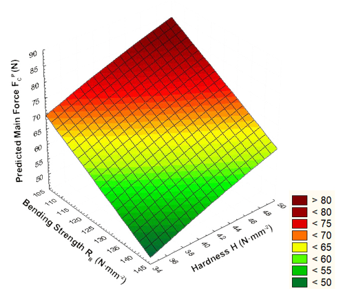
Fig. 7. Plot of the relationships among the predicted main force, F_C^P,H (N·mm^-2), and R_B (N·mm^-2), according to Eqs. 13 through 16; D₈=0.75 g·cm^-3; m_C =7.24 %; E =11355.13 N·mm^-2; γ_F=19.91^o; f_Z=0.427 mm; c_D = 3.25 mm

Figure 8 shows the relationships among the predicted main force, F_C^P, feed rate per tooth, f_Z, and oak wood modulus of elasticity, E. Figure 8 shows a strong, non-linear influence of f_Z on F_C^P. In the reference range, the overall increase was about 51 N. If the feed rate per tooth increase is 0.1 mm, the average increase in force F_C^P will be between 15.4 N and 19 N (lower values are valid for a lower modulus of elasticity, E. The influence of the modulus of elasticity, E, is much lower than the impact of f_Z and larger for a small feed rate per tooth, f_Z.

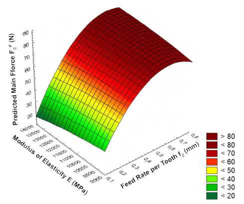
Fig. 8. Plot of the relationships among the predicted main force, F_C^P(N), c_D (mm), and E (N·mm^-2), according to Eqs. 13 through 16; D₈= 0.75 g·cm^-3; m_C = 7.24 %; H=46.14 N·mm^-2; R_B= 122.47 N·mm^-2; γ_F=19.91^o

Figure 9 shows the relationships between wood density, D, and moisture content, m_C, and the predicted main force, F_C^P.

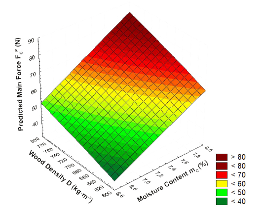
Fig. 9. The plot of the relationships between the predicted main force, F_C^P (N) and D (kg·m^-3) and m_C  (%), according to Eqs. 13 -16; H=44.16 MPa; R_B= 122.47 MPa; E= 11355.13 MPa; f_Z= 0.427 mm; g_F= 19.91^o; c_D= 3.25 mm

From Fig. 9 almost linear relations can be seen between F_C= f(D) and F_C= f(m_C). The predicted main cutting force F_C^P depends on the increase in D and m_C.  If the m_C  increase is 0.1 %, the average increase in force, F_C^P, will be around 2 N. If the D increase is 10 kg·m^-3, the average increase in force, F_C^P, will be around 0.8 N.

The value of the main predicted cutting force, F_C^P, (average in one cutting cycle), calculated from Eq. 11 through 16, evaluated for the following average parameters D= 750 kg·m^-3, m_C= 7.24%, H= 44.16 MPa, R_B= 122.47 MPa, and E= 11355 MPa, f_Z= 0.427 mm, c_D= 3.25 mm, g_F= 19.91⁰, was F_C=69.97 N. The F_C values calculated from formulas published in the studies Orlicz (1984), Amalitskij & Lûbčenko (1977), Beršadskij (1967) and Orlicz (1982) (f_Z, c_D) were higher 95%, higher 85%, lower 12% and higher 38%,  respectively. It has to be mentioned that the average values of D, H, R_B and E taken from the study Wagenfür & Scheiber (1974) were 8% lower, 21% lower, 28% higher and 11% higher, respectively. It can be seen from this comparison that the values of F_C obtained in the present study lie between the values evaluated with use of formulas published in the literature.

CONCLUSIONS

The analysis of results of the calculations performed makes it possible to state the following:

1. An increase in cutting depth, c_D, increased the main cutting force, F_C^P, in a parabolic, increasing manner, starting from about c_D= 3 mm.
2. The established relationshipF_C^P= f(c_D) was the strongest for the small rake angle, g_F, of 16°.
3. A decrease in rake angle, γ_F, for the highest examined cutting depth, c_D, of 4.5 mm increased the main cutting force, F_C, in a parabolic, decreasing manner. A further decrease in c_D up to c_D = 3 mm, resulted in a decrease in the relationship F_C^P= f(γF), with a minimum for γ_F ~21.4° at c_D = 2.5 mm.
4. An increase in bending strength, R_B, decreased the main cutting force, F_C^P, in an almost linear manner, but had a lower impact on it than Brinell hardness, H.
5. An increase in Brinell hardness, H, increased the main cutting force, F_C^P, in an almost linear manner.
6. An increase in cutting depth, c_D, increased the main cutting force, F_C^P, in a parabolic, decreasing manner.
7. An increase in the modulus of elasticity, E, decreased the main cutting force, F_C^P, in an almost linear manner.

ACKNOWLEDGMENTS

This research was realized as a part of the project “Studying climate change and its influence on the environment: impacts, adaptation and mitigation” (43007) financed by the Ministry of Education and Science of the Republic of Serbia within the framework of integrated and interdisciplinary research for the period 2011-2014.

The authors are grateful for the support of the Poznań Networking & Supercomputing Center, Poznań, Poland for calculation grant no. 241.

REFERENCES CITED

Afanasev, P. S. (1961). “Derevoobrabatyvaûŝie stanki” (Woodworking machinery)Lesnaâ promyšlennost’, Moskva

Amalitskij, V. V., and Lûbčenko, V. I. (1977). “Stanki i instrumenty derevoobrabatyvaûŝh predpriâtij” (Machinery and tools of woodworking factories)Lesnaâ promyšlennost’, Moskva

Axelsson, B., Lundberg, S., and Grönlund, A. (1993). “Studies of the main cutting force at and near a cutting edge,” Holz als Roh-und Werkstoff 51(1), 43-48. DOI: 10.1007/BF02764590

Beršadskij, A. L. (1967). “Razčet režimov rezaniâ drevesiny” (Resolution of modes of wood machining), Lesnaâ promyšlennost’, Moskva

Cristóvão, L., Broman, O., Grönlund, A., Ekevad, M., and Sitoe, R. (2012). “Main cutting force models for two species of tropical wood,” Wood Materials Science & Engineering. 7(3), 143-149. DOI: 10.1080/17480272.2012.662996

Deševoy, M. A. (1939). “Mehaničeskaâ tehnologiâ dereva” (Mechanical technology of wood)Lesotehničeskaâ Akademiâ, Leningrad

Ettelt, B., and Gittel, H. J. (2004). Sägen, Fräsen, Hobeln, Bohren, DRW -Verlag

Eyma, F., Méausoone, P, and Martin, P. (2004). “Study of the properties of thirteen tropical wood species to improve the prediction of cutting forces in mode B,” Annals of Forest Science 61(1), 55-64. DOI: 10.1051/forest:2003084

Franz, N. (1958). An Analysis of the Wood-Cutting Process, The Engineering Research Institute, Ann Arbor, MI

Feomentin, G. (2007). “Turning – Cutting forces and power measurements: Comparison of dynamometer force, electrical power and torque current,” COST Action E35, Training School: On- line control and measurements during cutting process, December 5-7, LABOMAP, ENSAM Cluny

Goglia, V. (1994). “Strojevi i alati za obradu drva I,” University of Zagreb, Faculty of Forestry, Zagreb, 40-78

Kivimaa, E. (1950). “Cutting Force in Woodworking,” VTT Julkaisu, Helsinki, Finland.

Koch, P. (1964): “Wood Machining Process,” Ronald Press Co., New York

Krzysik, F. (1975). “Nauka o drewnie” (Wood Science), Państwowe Wydawnictwo Naukowe, Warszawa 1975 (in Polish)

Mandić, M., Mladenović, G., Tanović, Lj., and Danon, G. (2014). “The predictive model for the cutting force in peripheral milling of oak wood,” Proc. of the 12th International Conference on Maintenance and Production Engineering KODIP, June 18-21, Budva, Montenegro, pp. 231-238

Manžos, F. M. (1974). “Derevorežuŝie stanki,” (Wood Cutting Machinery), Lesnaâ promyšlennost’, Moskva

McKenzie, W. (1960). Fundamental Analysis of the Wood-Cutting Process, Industry Program of the College of Engineering, Michigan

McKenzie, W. M., Ko, P., Cvitkovic, R., and Ringler, M. (1999). “Towards a model predicting cutting forces and surface quality in routing layered boards,” Proc. of the 14^th IWMS, pp. 489-497

Naylor, A., and Hackney, P. (2013). “A review of wood machining literature with a special focus on sawing,” BioResources 8(2), 3122-3135. DOI: 10.15376/biores.8.2.3122-3135

Orlicz, T. (1982). “Obróbka drewna narzędziami tnącymi,” (Machining of wood with use of cutting tools), in: Study book SGGW-AR, Warsaw

Porankiewicz, B. (2014). “Wood machining investigations: Parameters to consider for thorough experimentation,” BioResources 9(1), 4 -7. DOI: 10.15376/biores.9.1.4-7

Porankiewicz, B., Axelsson, B., Grönlund, A., and Marklund, B. (2011). “Main and normal cutting forces by machining wood of Pinus sylvestris,” BioResources 7(3), 2883-2894. DOI: 10.15376/biores.7.3.2883-2894

Scholz, F., Duss, M., Hasslinger R. J., and Ratnasingam, J. (2009). “Integrated model for the prediction of cutting forces,” Proc. of the 19^th IWMS, October 21-23, Nanjing, China, pp. 183 -190

SRPS D.A1.044 (1979) according to: ISO 3131:1975 ISO/TC 218, “Wood -Determination of density for physical and mechanical tests,” Serbian standard.

SRPS D.A1.046 (1979) according to: ISO 3133:1975 ISO/TC 218, “Wood – Determination of ultimate strength in static bending,” Serbian standard

Time, J. (1870). “Soprotivlene metallov i dereva rezaniû), Dermacow Press House, St. Petersburg, Russia

Tröger, J., and Scholz, F. (2005). “Modelling of cutting forces,” Proc. of the 17^th IWMS, Rosenheim, Germany

UNE-EN 1534 (2011). “Wood and parquet flooring. Determination of resistance to indentation (Brinell). Test method,” European Committee for Standardization, Brussels, Belgium

Wagenführ, R., Scheiber, C. (1974). “Holzatlas,” VEB Fachbuchverlag, Leipzig, (in German)

Woodson, G. E., and Koch, P. (1970). “Tool forces and chip formation in orthogonal cutting of loblolly pine,” Southern Forest Experiment Station, Forest Service, Dept. of Agriculture, New Orleans, LA.

Article submitted: January 14, 2015; Peer review completed: April 19, 2015; Revised version received: May 7, 2015; Accepted: July 9, 2015; Published: July 17, 2015.

DOI: 10.15376/biores.10.3.5489-5502

APPENDIX

ERRATUM: An Attempt at Modelling of Cutting Forces in Oak Peripheral Milling (BioResources 10(3), 5489-5502)

Marija Mandić,^a Bolesław Porankiewicz,^b,* and Gradimir Danon ^a

Contact information: a: Department of Wood Processing, University of Belgrade- Faculty of Forestry, Belgrade, Serbia; b: Poznań University of Technology, Poland;

*Corresponding author: poranek@amu.edu.pl

Article submitted: January 14, 2015; Peer review completed: April 19, 2015; Revised version received: May 7, 2015; Accepted: July 9, 2015; Published: July 17, 2015.

DOI: 10.15376/biores.10.3.5489-5502

The authors have extended and improved the statistical model, which impacts the results of the published paper. What follows are the corrected portions of the manuscript.

Abstract

Two parameters were added to the second sentence: density, D, and moisture content, m_C. The last sentence of the abstract section has been revised: Several interactions between the machining parameters and properties of wood were confirmed in the developed relationship F_C= f(D, m_C, H, R_B, E, f_Z, c_D, γ_F).

Experimental

In the fourth sentence of the third paragraph, the value of the radius of the edges round up was corrected r= 2 mm. In the second paragraph on the sixth page and seventh page of the article the number of experimental matrix changed from 25 to 22 data points.

Results and Discussion

In the first paragraph the number of iterations was changed from 2.84·10¹⁰ to 7.54·10⁹

The following paragraph has been revised:

The following estimators were evaluated: e1= 0.68806; e2= 0.62019; e3= 0.18212; e4= 0.045741; e5= 0.27236; e6= 0.53737; e7= 0.54972, e8= -0.50384; e9= 106.55693; e10= -14.2737; e11= -1.80803; e12= -7.0966•10-3; e13= -7.53491•10-6; e14= -0.056067; e15= 0.038487; e16= 0.01174; e17= -14.60027.

The third and the fourth paragraph has been revised:

The rounding of the estimator values to the 5th decimal place produced an acceptable deterioration of the fit 0.005%. Reducing the number of the rounded decimal digits to 4, 3, 2 and 1 would cause unacceptable deterioration of the fit as much as 15%, 85%, 96% and 3927%, respectively.

The coefficients of relative importance, CRI, for the estimators have the following values: CRI1=159517; CRI2=816197; CRI3=404687; CRI4=63793; CRI5=1383657; CRI6= 725575; CRI7=1070522; CRI8=815139; CRI9=764929; CRI10=572373; CRI11=313681; CRI12= 9737; CRI13=127516; CRI14=10564; CRI15=36463; CRI16=1629705; CRI17=6637.

In the fifth paragraph on the seventh page of the article the number of experimental matrix was changed from 25 to 22 data points. In the last sentence of this paragraph the values of the quantifiers were changed from S_K= 61.86, R= 1.00, R²= 0.99, and S_R= 1.76 to S_K= 70.94; R= 0.995; R²= 0.991; and S_R= 1.88.

Equations 14 through 16 were updated:

A=0.01174·D^0.68806·m_C^0.62019·H^0.18212·R_B^0.045741·E^0.27236·f_Z^0.53737·γ_F^0.54972·c_D^-0.50384       (14)

B=106.55693·f_Z·c_D – 14.2737·f_Z·γ_F – 1.80803·R_b·f_Z – 7.0966·10^-3 · R_B·g_F       (15)     

C=-7.53491·10^-6· D ·E – 0.056067 · D · f_Z + 0.038487 · R_B  -14.60027        (16)

In the last paragraph of the eighth page values S_R was corrected from S_R=4.79 N to S_R= 5.27 N.

Figure 5 was updated to:

Fig. 5. The plot of the observed main force F_C^O against the predicted F_C^P values, according to Eqs. 13 through 16

The first paragraph on the ninth page has been revised: Figure 6 shows a plot of the relationships among the main cutting force, F_c^P, the cutting depth, c_D,  and the rake angle, g_F. Figure 6 shows that F_C^P strongly, non-linearly  depends on c_D in a parabolic decreasing manner. An increase in c_D increased F_C^P, more for a lower g_F. The average change of F_C^P with an increase in the cutting depth, c_D,  by 0.1 mm is between 4 N and 2.6 N, depending on the size of the rake angle, g_F. An increase in g_F increases F_C^P for the largest cutting depth, c_D. As c_D fell below ~3 mm, a minimum started to appear. For the lowest c_D, the influence of g_F on F_C^P was small, with a minimum at g_F ~21.4° at c_D = 2.5 mm. The relationship F_C^P = f(c_D) combines the influence of increasing cutting layer thickness (chip thickness), a_p,  and to a lesser degree the influence of increasing grain orientation angle, j_V.

Figure 6 was changed to:

Fig. 6. The plot of the relationships among the predicted main force F_C^P (N), g_F (^o), and c_D (mm), according to Eqs. 13 -16; D= 750 kg·m^-3; m_C= 7.24 %; H= 44.16 MPa; R_B= 122.47 MPa; E= 11355.13 MPa;  f_Z= 0.427 mm

The last three sentences in the first paragraph of the tenth page have been revised: From Fig. 7, it can be seen that the influence of Brinell hardness, H, on F_C^P was higher than that of bending strength, R_B. When bending strength, R_B, increases by 10 MPa, the average cutting force will be lower by as much as 5.6 N. In the case of an increase in hardness, H, by 10 MPa the cutting force grows by 9.4 N.

Figure 7 was updated to:

Fig. 7. The plot of the relationships among the predicted main force, F_C^P, H (MPa) and R_B (MPa), according to Eqs. 13 -16; D= 750 kg·m^-3; m_C= 7.24 %; E= 11355.13 MPa; g_F= 19.91^o; f_Z= 0.427 mm; c_D= 3.25 mm

The last paragraph of the tenth page has been revised: Fig. 8 shows the relationships among the predicted main force, F_C^P, feed rate per tooth, f_Z, and oak wood modulus of elasticity, E. Figure 8 shows a strong, non-linear influence of f_Z on F_C^P. In the reference range, the overall increase was about 51 N. If the feed rate per tooth increase is 0.1 mm, the average increase in force F_C^P will be between 15.4 N and 19 N (lower values are valid for a lower modulus of elasticity, E. The influence of the modulus of elasticity, E, is much lower than the impact of f_Z and larger for a small feed rate per tooth, f_Z.

Figure 8 was changed to:

Fig. 8. The plot of the relationships among the predicted main force, F_C^P (N), f_Z (mm), and E (MPa), according to Eqs. 13 -16; D= 750 kg·cm^-3; m_C = 7.24 %; H= 44.16 MPa; R_B= 122.47 MPa; c_D= 3.25 mm; g_F= 19.91^o

After Figure 8, the following sentence: Figure 9 shows the relationships between wood density, D, and moisture content, m_C, and the predicted main force, F_C^P, has been added and is followed by Fig. 9:

Fig. 9. The plot of the relationships between the predicted main force, F_C^P (N) and D (kgm^-3) and m_C (%), according to Eqs. 13 -16; H=44.16 MPa; R_B= 122.47 MPa; E= 11355.13 MPa; f_Z= 0.427 mm; _F= 19.91^o; c_D= 3.25 mm

The first paragraph on the twelwth page has been added: From Fig. 9 almost linear relations can be seen between F_C= f(D) and F_C= f(m_C). The predicted main cutting force F_C^P depends on the increase in D and m_C.  If the m_C increase is 0.1 %, the average increase in force, F_C^P, will be around 2 N. If the D increase is 10 kg·m^-3, the average increase in force, F_C^P, will be around 0.8 N.

In the last paragraph the values of F_C was corrected from F_C=77.7N to F_C=69.97 N. The following sentence revised to: The F_C values calculated from formulas published in the studies Orlicz (1984), Amalitskij and Lûbčenko (1977), Beršadskij (1967) and Orlicz (1982) (f_Z, c_D) were higher 95%, higher 85%, lower 12% and higher 38%, respectively. 

Conclusions

Conclusions under the ordinal number 1, 3, 4, 5 and 7 are revised to:

1. An increase in cutting depth, c_D, increased the main cutting force, F_C^P, in a parabolic, increasing manner, starting from about c_D= 3 mm.
2. A decrease in rake angle, g_F, for the highest examined cutting depth, c_D, of 4.5 mm increased the main cutting force, F_C,  in a parabolic, decreasing manner. A further decrease in c_D up to c_D= 3 mm, resulted in a decrease in the relationship F_C^P= f(g_F), with a minimum for g_F ~21.4° at c_D= 2.5 mm.
3. An increase in bending strength, R_B, decreased the main cutting force, F_C^P, in an almost linear manner, but had a lower impact on it than Brinell hardness, H.
4. An increase in Brinell hardness, H, increased the main cutting force, F_C^P, in an almost linear manner.
5. An increase in the modulus of elasticity, E, decreased the main cutting force, F_C^P, in an almost linear manner.

We apologise to the readers of the journal for any inconvenience.