Comparative analysis of the elastic constants measured via conventional, ultrasound, and 3-D digital image correlation methods in Eucalyptus globulus

Abstract

Full Article

Comparative Analysis of the Elastic Constants Measured via Conventional, Ultrasound, and 3-D Digital Image Correlation Methods in Eucalyptus globulus Labill

Jorge Crespo,^a,* José Ramón Aira,^b Carlos Vázquez,^a and Manuel Guaita ^a

The design of engineering high value-added products and timber structures analysis requires reliable elastic characteristics related to a theoretical model that describes the elastic behavior of wood material. The present research focuses on determining the elastic constants of Eucalyptus globulus Labill., which allow their implementation as input parameters in any numerical model. The great potential of this species for novel structural applications was considered due to its superior mechanical properties. Two different testing methods were applied to the same specimens to directly compare the results. These two tests were conventional mechanical compression and a non-destructive ultrasound procedure. In addition, two different strain measurement techniques were contrasted in the performance of the mechanical tests, namely the conventional strain gauges that give local measurements, and the 3-D full-field optical system based on the principles of digital image correlation. The elastic values obtained via ultrasound are higher than those coming from mechanical testing using conventional gauges. Conventional gauges lead to underestimated values in comparison to the results from full-field strain measurements. Eucalyptus globulus shows greater longitudinal and transversal stiffness than the average values for other hardwoods, which verifies the good structural possibilities of this species.

Keywords: Eucalyptus globulus; Orthotropic characterization; Ultrasound; Mechanical tests; DIC

Contact information: a: Department of Agroforestry Engineering, Higher Polytechnic School of Lugo, University of Santiago de Compostela, Lugo, Spain; b: Department of Agricultural and Forestry Engineering, University of Valladolid, Valladolid, Spain;

*Corresponding author: jorge.crespo@usc.es

INTRODUCTION

Plantations of white eucalyptus (Eucalyptus globulus Labill.) cover a large area within the southern European Atlantic climate. In Spain, in the Galicia region, and Portugal they form a coastal strip containing the most productive forests in Europe. The total area covered by white eucalyptus is gradually increasing and now spans across 383,000 hectares in Galicia, according to data from the Third National Forestry Inventory (IFN III 2007). Eucalyptus wood is mainly used for power generation and as a source of fiber for the cellulose industry. Nevertheless, several studies in recent years have shown its great potential for the development of high added-value processed products (e.g. Lara-Bocanegra et al. 2017).

The advantages of its fast growth cycle, high mechanical strength, and high structural stiffness of eucalyptus wood make it a very competitive structural material, and of recent research interest. For example, the FAIR CT 98-9579 (2001) project studied some of the properties of eucalyptus wood from Galician trees aged from 23 years to 35 years. The mean values that corresponded to several physical-mechanical properties were obtained, including density (760 kg/m³), longitudinal elasticity modulus (20580 N/mm²), bending strength (130 N/mm²), and compression strength parallel to the grain (71 N/mm²), all of which indicate superior structural possibilities of this species. The structural classification of Spanish E. globulus (Labill.) was performed by the CIFOR-INIA laboratory according to the guidelines of the EN 384 (2004) (Fernández-Golfín et al. 2007). The standard UNE 56546 (2013) sets an MEF (Hardwood structural timber) visual quality that corresponds to the D40 strength class according to EN 1912 (2013).

When considering engineering applications, macroscopic material models are essential for numerical structural analyses through the finite element (FE) method (Schmidt and Kaliske 2009). The engineering parameters defining these models are the elastic constants that must accurately reflect the wood behavior described as linear-elastic in the small strain regime (Gibson and Ashby 2001).  Although wood is an anisotropic material, it is usually simplified in mechanical analysis as orthotropic with three planes of symmetry that is defined by three main directions: longitudinal (L), radial (R), and tangential (T). These material assumptions have been consistently established in previous studies (Mascia 2003; Mascia and Lahr 2006). The characterization of the linear elastic orthotropic behavior of clear wood requires the determination of 12 elastic constants that form the stiffness matrix. The stiffness matrix consists of 3 longitudinal elasticity moduli (E_L, E_R, E_T), 3 shear elasticity moduli (G_LR, G_LT, G_RT), and 6 Poisson’s ratios (υ_LR, υ_RL, υ_LT, υ_TL, υ_RT, and υ_TR). These parameters can be reduced to 9 independent values when symmetry conditions in the stiffness matrix are applied; therefore, its determination becomes fundamental work.

Conventionally, this set of material parameters is experimentally determined by performing mechanical tests in which both the loading and specimen geometry are typically oriented along the material directions (Sliker et al. 1994; Aira et al. 2014). However, there is currently an increasing use of non-destructive techniques to this end, including methods like ultrasound (Gonςalves et al. 2001, 2011a, 2011b, 2014; Hering et al. 2012). Additionally, the strain measuring devices are also improving. This initiates an emerging tendency to use optical methods that provide full-field results. Optical methods also allow for inhomogeneous assumptions of the stress/strain states across the specimen, which are characteristic of materials with such complex heterogeneities, such as wood (Avril et al. 2008; Dahl and Malo 2009; Majano-Majano et al. 2012; Xavier et al. 2012). These methods also have the advantage of having no physical contact with the specimen, thereby avoiding any possible mechanical influence.

The present study focuses on determining the elastic constants of E. globulus, which define its behavior to allow its implementation in any numerical model. The two different methodologies used for this purpose to compare the results were ultrasound wave propagation and mechanical compression testing. Additionally, two different techniques have also been compared for the strain measurements during the performance of the mechanical tests: conventional, simple, and double gauges, and the 3-D stereovision optical system, based on the principles of digital image correlation (DIC). 

EXPERIMENTAL

Materials

The raw material consisted of 20 high visual-quality boards made of E. globulus (Labill.) from Galicia. The boards followed a MEF visual grade according to UNE 56546, corresponding to a D40 strength class. These boards had nominal dimensions of 20 mm x 80 mm x 3000 mm, and did not present major defects like knots or noticeable twists or bow deformations.

Prior to the specimen’s preparation, these boards were conditioned in a conditioning chamber at a temperature of 20 ºC ± 2 ºC and 65% ± 5% relative humidity, according to the ISO 3129 (2012). It resulted in an average moisture content of 10.8%.

Six small prismatic specimens were cut from each board following the orientations represented in Fig. 1, which resulted in a total of 120 specimens. Three of these specimens were oriented following the main orthotropic directions: longitudinal (L), radial (R), and tangential (T) (specimens 1, 2, and 3, respectively). The other three specimens were oriented 45º to the LR (longitudinal-radial), LT (longitudinal-tangential), and RT (radial-tangential) planes (specimens 4, 5, and 6, respectively). The same specimens were first tested via ultrasound and afterwards by mechanical compression, which measured the strains by gauges to obtain a direct comparison of the results.

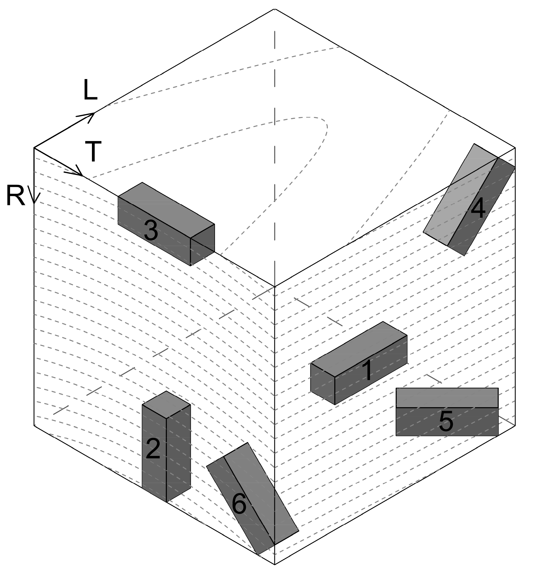
Fig. 1. Layout of the specimen orientations

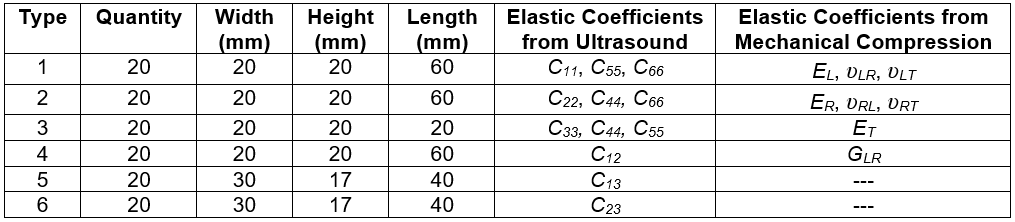
Following the ultrasound and mechanical procedures, the dimensions and elastic constants evaluated from each of the 6 specimen types are compiled in Table 1.

Table 1. Specimen Dimensions and Elastic Coefficients Obtained

For optical measurement analysis, 10 of the total 20 boards were used to produce another set of specimens with the same dimensions as specified in Table 1. 

Methods

Ultrasound tests

To perform the ultrasound tests, an Olympus Epoch 600 (Hamburg, Germany) portable device was used (Fig. 2). This was equipped with longitudinal and transversal Panametrics-NDT Olympus plane transducers, both with 1.0 MHz nominal frequency and a 15-mm external diameter. The longitudinal transducers emitted a single longitudinal wave, which propagated and polarized directionally towards emission (between the two transducers). The transversal transducers released a longitudinal wave that propagated and polarized directionally towards emission together with another transversal wave that propagated directionally towards emission and polarized in the perpendicular direction.

To improve the coupling as much as possible, pure starch glucose was used as the couplant gel between the transducers and the specimens to help keep constant pressure throughout measuring (Gonçalves et al. 2011a).

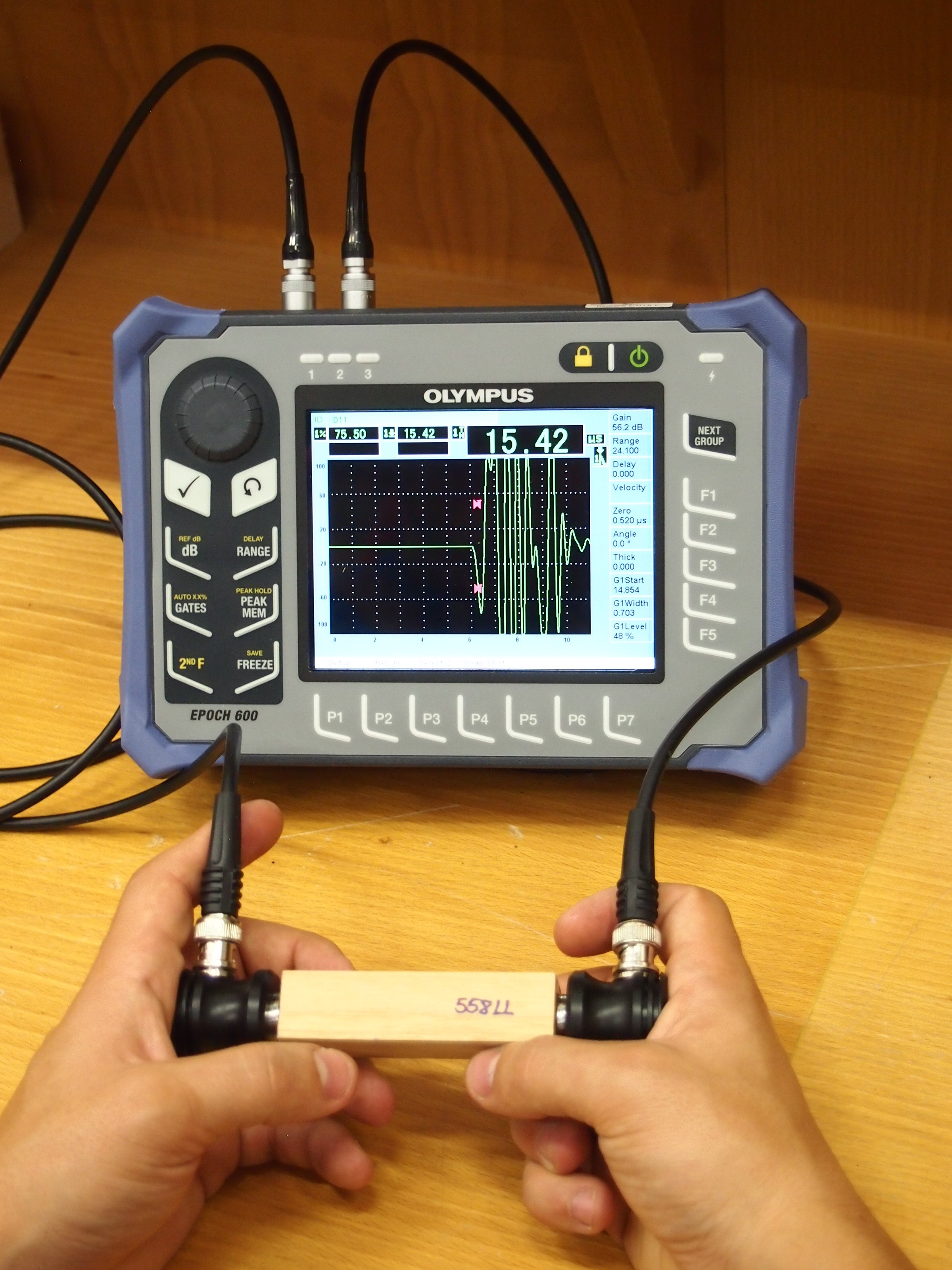
Fig. 2. Ultrasound test device

Although signal attenuation is reduced within the wood of small specimens, previous studies have shown that to approach the hypothesis of wave propagation in an infinite medium, the distance between the transducers must be greater than the wavelength (λ). Therefore, specimens that were longer than 3 λ to 5 λ were suitable (Bucur 2006; Trinca and Gonçalves 2009). In the present study, the distance between transducers was greater than 7 λ for all of the specimens and measurement directions (Table 1).

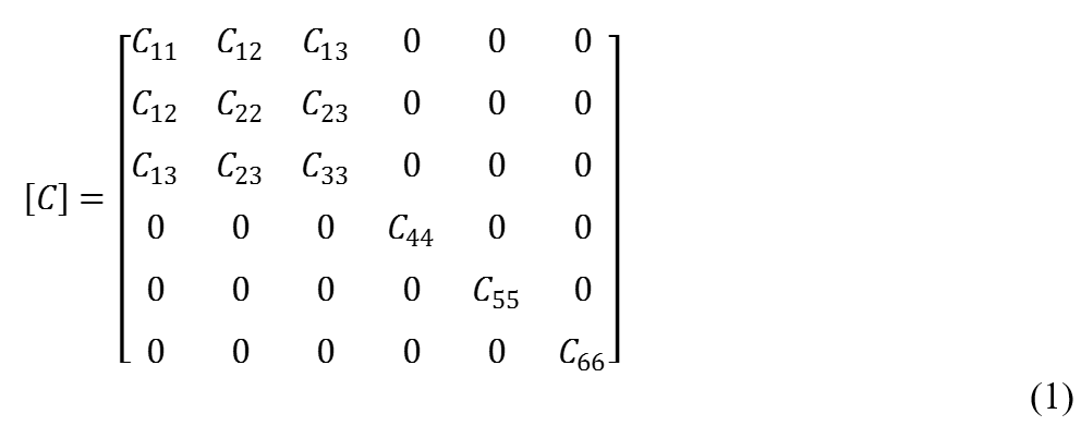
The elastic constants were obtained following the procedure described by Gonçalves et al. (2011b) and applied also by Vázquez et al. (2015). When waves propagate within a three dimensional body it is necessary to calculate all of the elements of the stiffness matrix [C] (Eq. 1). The reason for this is because the rest of the elastic properties of the body affect wave propagation along one direction. Ozyhar et al. (2013) concluded that obtaining the stiffness matrix when taking into account only the terms along the main diagonal of the matrix led to an over-estimation of the longitudinal and transversal elastic moduli.

The terms of the main diagonal of [C] were determined by using both longitudinal and transversal waves, placing the transducers at different positions respecting the axes of the material, and applying Christoffel’s tensor equations, which relate the elasticity theory and wave propagation theory (Bucur 2006). These test configurations, and the corresponding mathematical expressions (Eqs. 2 to 7), are summarized in Table 2 (Gonçalves et al. 2014).

Table 2. Determination of the Diagonal Terms of the Stiffness Matrix [C]

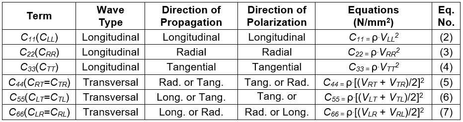
In Eqs. 2-7 (Table 2), ρ denoted the material density (kg/m³) and V the wave velocity (m/s), which was derived from the duration of the wave propagation and the length of the specimen in each test. The first subscript of the latter corresponded to the direction of propagation and the second with the direction of polarization. Therefore, V_LL, V_RR, and V_TT, were the velocities of the longitudinal waves measured in the three axial directions. Furthermore, V_RT, V_TR, V_LT, V_TL, V_LR, and V_RL, were the velocities of the transversal waves measured in the axial directions with polarization along the perpendicular axes.

The off-diagonal terms of the matrix [C] were determined from the expressions below (Eqs. 8 to 10), derived from Christoffel’s tensor. Transversal transducers were used in these cases, emitting quasi-transverse waves measured with a 45º angular displacement within the corresponding orthotropic plane (LR, LT, or RT), and polarizing in such plane. According to Bucur and Archer (1984), 45º angles led to the smallest relative error.

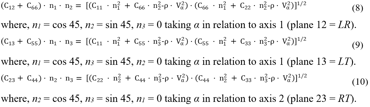
where, n₂ = cos 45, n₃ = sin 45, n₁ = 0 taking α in relation to axis 2 (plane 23 = RT).

In equations 8, 9, and 10, V_α corresponded to the wave velocity propagating in α direction. Thereby, V_QLR, V_QLT, and V_QRT denoted the velocity of a quasi-transversal wave propagating in a direction of 45º to the orthotropic axes of the corresponding plane (LR, LT, or RT). Once all of the stiffness matrix terms were obtained, the compliance matrix [S] was determined by directly calculating its inverse, [C]^-1 = [S] (Eq. 11).

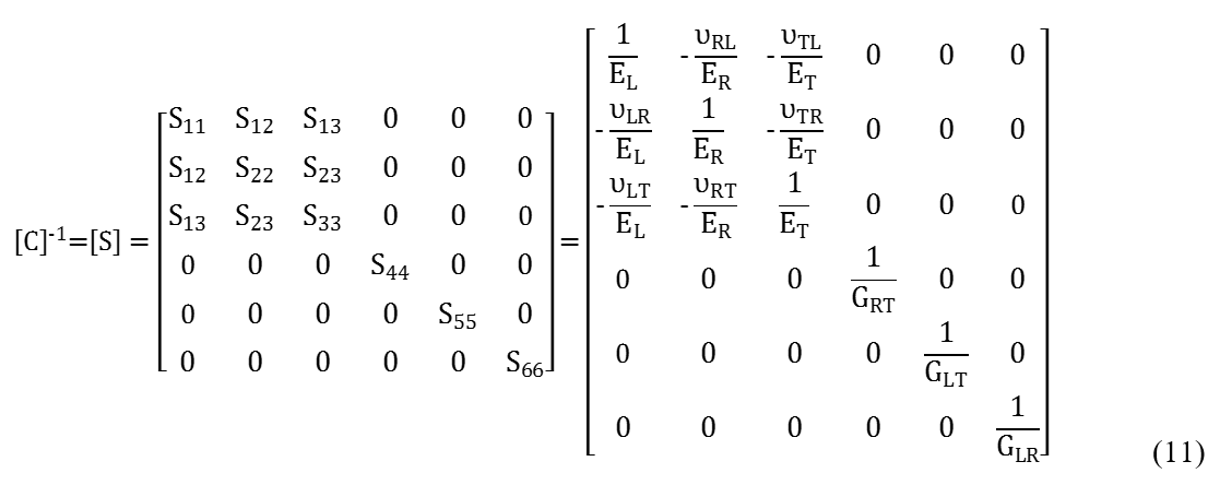
The 12 elastic constants can be calculated from the compliance matrix [S] terms. The Young’s modulus, E_L, E_R, and E_T were in the longitudinal, radial, and tangential directions, respectively. The shear modulus, G_RT, G_LT, and G_LR were in the radial-tangential, longitudinal-tangential, and longitudinal-radial planes, respectively. The Poisson’s ratios were υ_LR, υ_LT, υ_RT, υ_RL, υ_TL, and υ_TR for each of the planes.

This portion of the research was performed at the Laboratory of Engineering Timber Structures (PEMADE) in the University of Santiago de Compostela. 

Compression tests with mechanical measurements

The small clear specimens used in the ultrasound study were also subjected to mechanical compression testing. The upper plate of the testing equipment was coupled to a loading cell of 50 kN, while the lower plate was fixed to a stationary metal frame so that both plates remained horizontal and parallel during the entire test (Fig. 3).

In the first batch of tests, the strains were measured by placing strain gauges directly onto the same specimens used previously for ultrasound testing (Fig. 3). The gauges responded to simple C2A-13-125LW-350 type with an effective length of 3.18 mm and an effective width of 1.78 mm. The gauges also responded to double rosettes C2A-13-125LT-350 type, each with an effective length of 3.18 mm, an effective width of 3.81 mm, and a sufficient sensitivity to measure deformation greater than 1·10^-6 m/m. A cyanoacrylate adhesive with less longitudinal stiffness than the wood material was used to prevent restrictions on the specimen deformation by receiving the external load. This adhesive also showed high transversal stiffness so that the deformation of the strain gauge was not dampened by the thickness of the adhesive (Aira et al. 2014).

Six different mechanical tests were performed: compression parallel to the grain and applying the load along the longitudinal direction (Fig. 3a); compression perpendicular to the grain with the load in the radial and tangential directions (Fig. 3b); and oblique compression by applying the load at an angle of 45º to the three grain directions, respectively (Fig. 3c). In each of these tests, the gauges were placed onto the specimen according to different arrangements, in or out, of the axes depending on the elastic constant, determined according to Fig. 4.

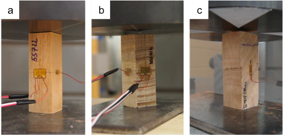
Fig. 3. Example of measurements mechanical tests. (a) Compression parallel to the grain; (b) compression perpendicular to the grain; (c) and oblique compression

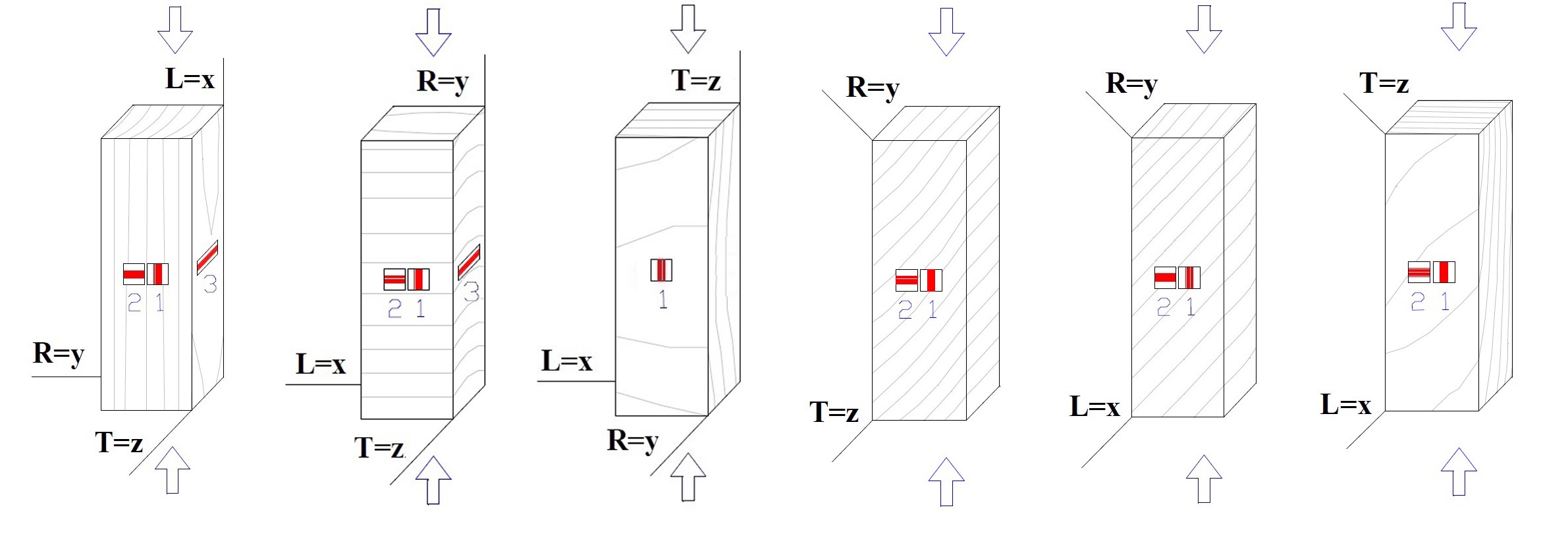
Fig. 4. Schemes of strain gauge arrangement in each type of mechanical test

In particular, compression parallel to the grain was performed according to ISO 13061 (2014) (Part 17) under a load velocity control of 170 N/s. On each test specimen, a double rosette (vertical according to direction L and horizontal according to direction R) was placed on the front face, and a single gauge (horizontal according to direction T) on one of its lateral faces. For this arrangement, the elastic constants E_L, υ_LR, and υ_LT were obtained from the elastic range using the following relations, Eq. 12,

The tests in compression perpendicular to the grain loading along the radial axis were performed following the ISO 13061 (2014) standard (Part 5). The load was applied by means of a constant velocity control of 0.3 mm/min. Three strain gauges were placed on each of these test specimens, with a double rosette (vertical in direction R and horizontal in direction L) on the front face and a single gauge (horizontal in direction T) on one of its lateral faces. The elastic constants E_R, υ_RL, and υ_RT were obtained using the following expressions in Eq. 13,

Regarding the tests of compression perpendicular to the grain loading in the tangential direction, it was only possible to attach one vertical strain gauge in the tangential direction because of the specimen’s dimensions. The longitudinal modulus of elasticity E_T was obtained according to Eq. 14,

Oblique compression tests were performed using specimens with an inclination of the grain of 45º to the load direction. A double rosette was placed on the front face of each specimen (horizontal and vertical). Due to the small dimensions of the specimens, it was possible to test along the shear plane LR. The elastic constant G_LR was obtained using Eq. 15,

Compression tests with stereovision measurements

Additionally, more compression tests were performed using a 3-D optical system for the strain measurements, ARAMIS® 3D (GOM, Braunschweig, Germany) (Fig. 5). This system applies the principles of digital image correlation (DIC) and possess clear advantages in comparison with the use of strain gauges like the obtainment of full-field measurements and not solely directionally, which is crucial for a non-homogeneous material. Full-field measurements are also advantageous for connecting the results with any macro-scale model. This technique also has the interest of being non-intrusive and requires simple specimen preparation (speckle pattern). In this study, the speckle pattern was performed via the application of a thin coating of white aerosol spray paint onto the specimen faces, followed by a spot distribution of black paint (Fig. 5).

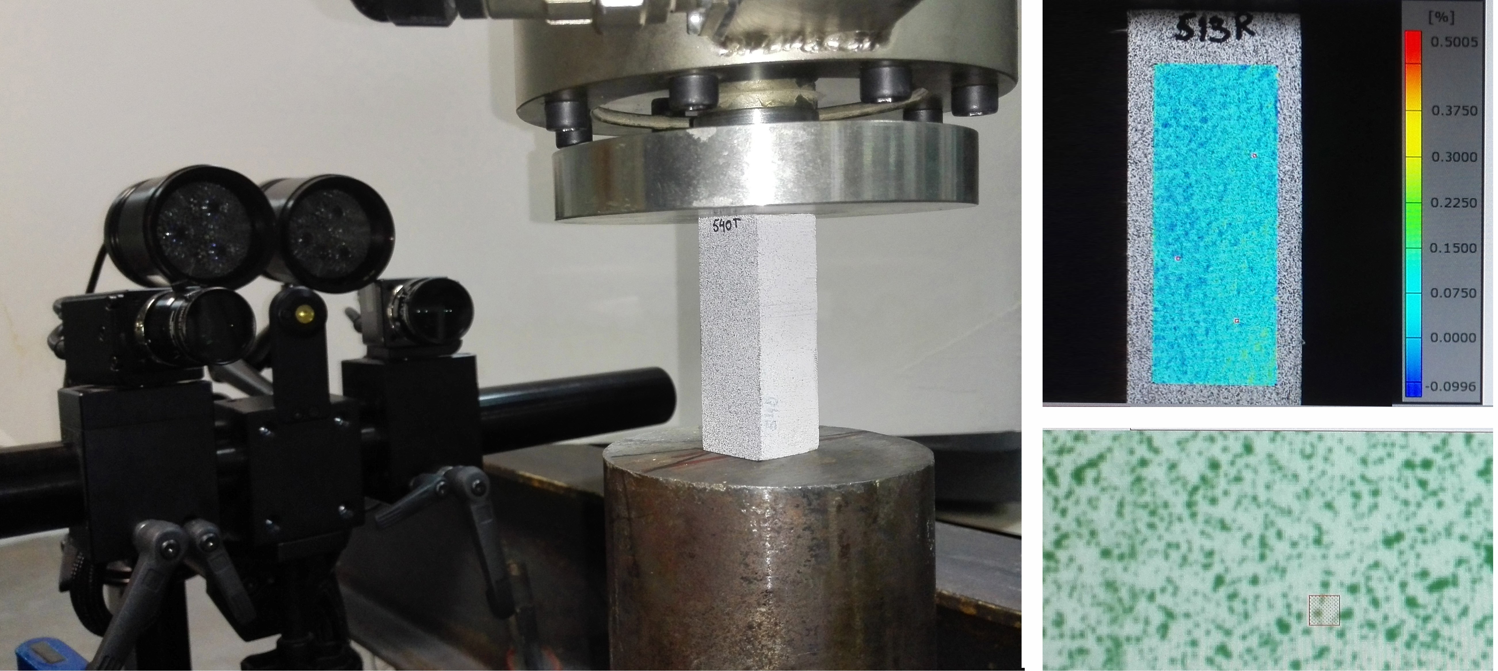
Fig. 5. Testing set-up with ARAMIS 3D and speckle pattern of the specimens

In the DIC method, the displacement field was measured by analyzing the geometrical deformation of the images of the surface of interest. The images were recorded before and after deformation by two CCD cameras (5 Megapixels resolution) (GOM, Braunschweig, Germany). For this purpose, the initial undeformed image was mapped by the correlation of windows (facets) formed by a group of pixels, within which an independent measurement of the displacement was calculated.

A stereovision angle of 25º was set-up between the two cameras before calibration. A 35-mm lens and a reference field of view of 65 mm x 55 mm were selected. The base distance between cameras was set to 110 mm, which corresponded to a working distance of 340 mm. The depth of field was adjusted to 46 mm to image each pair of orthogonal adjacent faces of the prismatic specimen (Fig. 5).

For parameter measurements, a facet size of 15 pixels x 15 pixels was chosen as the region of interest for the size and the quality of the pattern. The facet step was set to 13 pixels x 13 pixels, which allowed for an overlapping of 2 pixels in order to enhance the spatial resolution. The in-plane displacements were then numerically differentiated to determine the strain field needed for the material characterization problem, on a base computation size of 5 subsets.

Every test was kept in the elastic range, which avoided failure to derive from the same specimen all of the possible elastic constants. For each loading direction, the specimens were placed on the testing machine in such a way that the deformation field at two adjacent faces could be measured simultaneously. During the tests, the cameras were triggered every second, while also logging the analogue signal readings of displacement and force from the loading machine during deformation of the specimen. They recorded synchronized stereo images of the patterned surface of these different loading stages. These were processed afterwards and the vertical and horizontal strains on the two visible faces of the specimens were obtained.

The stereovision measurements were performed at the Laboratory of Structures in the ETS Architecture, Technical University of Madrid.

RESULTS AND DISCUSSION

Ultrasound Parameters

From the ultrasound tests in hardwoods, an ultrasound wave propagating longitudinally followed the direction of the vessels (functioning as conductors) and the fibers (functioning as supports). The length-diameter ratio in these structures was high and they functioned as pipes adding continuity to the material, which favored an increase of the wave propagation velocity in this direction. Radially, the wave met the wood rays, which favored material continuity in this direction. On the contrary, there were no anatomical structures in the tangential direction, which favored the wave propagation that led to lower velocities than in the radial and longitudinal directions. Table 3 shows the wave propagation velocities for the different directions which, as they depend on the anatomy of the wood itself, must fulfill the following ratios: V₁₁ > V₂₂ > V₃₃ (5350 > 1992 > 1341, respectively) and V₆₆ > V₅₅ > V₄₄ (1432 > 1082 > 786, respectively).

Table 3. Average Wave Velocity (m/s)

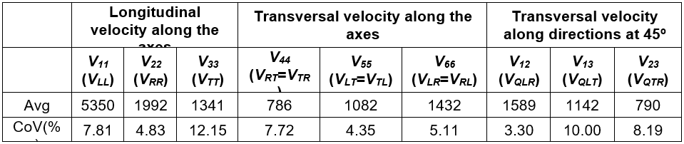
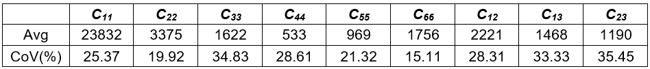
Table 4 shows the stiffness matrix coefficients [C] that were obtained. Its validation is undertaken by considering the theoretical bases of the acoustic behavior and the mechanical properties of the wood. In this way, the resulting values must fulfill the next relations: C₁₁ > C₂₂ > C₃₃ (23832 > 3375 > 1622, respectively), C₆₆ > C₅₅ > C₄₄ (1756 > 969 > 533, respectively), and C₁₂ > C₁₃ > C₂₃ (2221 > 1468 > 1190, respectively). 

Table 4. Stiffness Matrix Coefficients Obtained by Ultrasound Tests (N/mm²)

Stereovisions Measurements

From the stereovision measurements performed during the mechanical tests, 3-D coordinates were determined for each pair of images and then converted to relative displacements and strains. The 3-D device allowed the determination of the strains of two specimen faces simultaneously (Fig. 6).

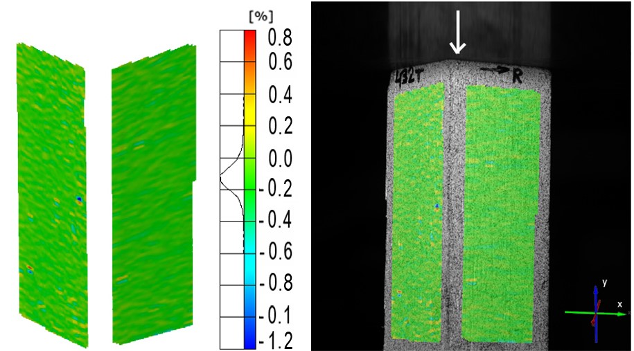
Fig. 6. Example of strain distribution in two faces of the specimen by the ARAMIS system

According to the defined procedure, the averaged values of the working area data were evaluated. Figure 7 shows an example of the longitudinal strains values in each of the three main directions, distributed in the specimen face when the load was applied parallel to the grain.

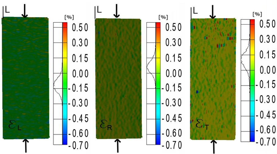
Fig. 7. Longitudinal, radial, and tangential strain distributions for a longitudinal load of 38 N/mm²

In the same way, Fig. 8 represents an example of the three strain distributions when the load was applied along the radial direction.

Fig. 8. Longitudinal, radial, and tangential strain distributions for a radial load of 6 N/mm²

The tangential and longitudinal strain distributions when the load was applied following the tangential direction are shown in Fig. 9.

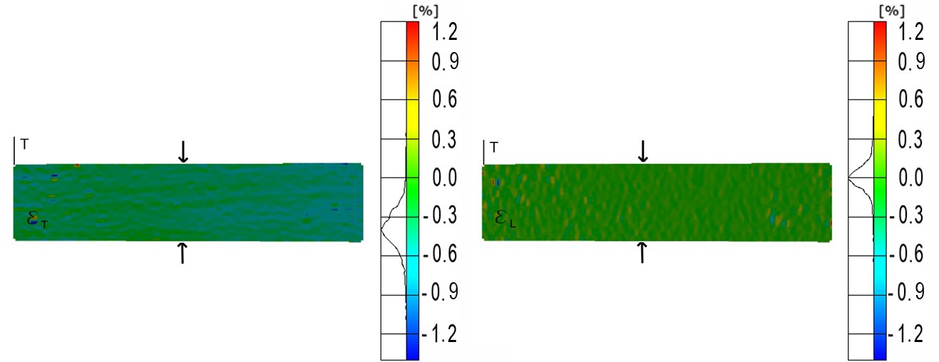
Fig. 9. Longitudinal and tangential strain distributions for a tangential load of 6 N/mm²

Figure 10 shows an example of the horizontal and vertical strain distributions that resulted from an oblique compression test along the shear plane LR, using specimens with a slope of the grain of 45º. Due to the restrictions of the small specimen dimensions, it was not possible to test along the other two shear planes.

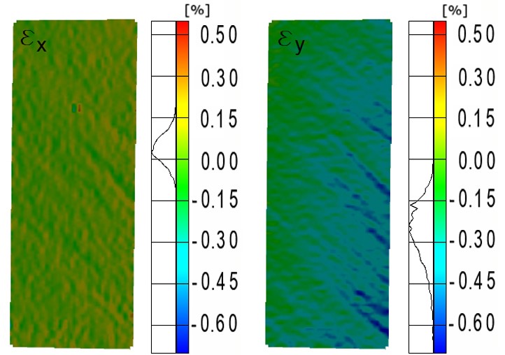
Fig. 10. Horizontal and vertical strain distributions for a 45º LR loading configuration at 10 N/mm²

Elastic Constants Results

Table 5 summarized the mean values and variation coefficients for the elastic constants obtained by ultrasound and mechanical tests. These values are also compared to those reported by Guitard (1987) for hardwoods with a medium density of 650 kg/m³. In the present study, the average density of the eucalyptus specimens was 854 kg/m³ with a variation coefficient of 14.90%. This value is similar to that stated at UNE 56546 (2013).

As can be seen, the elastic moduli of E. globulus were slightly higher than the references due to the higher density and subsequently greater stiffness (Guitard 1987). In contrast, the Poisson’s ratios were close to the reference values. Overall, the results were consistent and presented the usual variation coefficients in wood.

When the values obtained from ultrasound and mechanical tests were compared using strain gauges, it can be noted that the longitudinal elasticity moduli determined by the ultrasound were slightly higher than those resulting from the mechanical procedure. The greatest differences were found in the radial direction, especially in the tangential direction with lower values from the mechanical test using gauges. This may have been due to the influence of the curvature of the growth rings, which would have made the wood behave less like a theoretical orthotropic material. This may have affected the mechanical test measurements (Gonçalves et al. 2011b). Moreover, it can be observed that E_T obtained by ultrasound was similar to the reference value. This indicated that the measurement from the mechanical testing was influenced by the excessive closeness of the strain gauges to the compression plates, as the specimen dimensions were very small for this type of test. 

Table 5. Elastic Coefficients, Elasticity Moduli in N/mm², and Variation Coefficients in % in Brackets

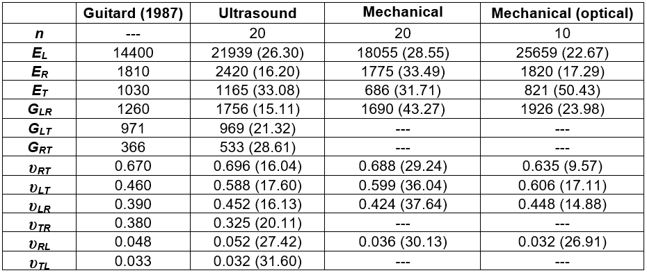
With respect to the values obtained from the stereovision measurements by ARAMIS®, all of the longitudinal moduli were higher than those that resulted from the mechanical gauge readings, but not as high as the values obtained by ultrasound (excluding E_L). Stereovision technique also provided the highest value of the only shear moduli measured, G_LR. Accordingly, the values of the elastic constants from local gauges measurements were usually underestimated in comparison to the results obtained from full-field strain measurements, which provided more realistic values.

Regarding CoV values, It seems to be significantly higher for mechanical measurements with gauges except for E_T.

In spite of the fact that ultrasound and mechanical methods are valid means of obtaining the material stiffness matrix, authors such as Preziosa (1982), Bucur (2006), and Gonçalves et al. (2001, 2011b, 2014) state that they expect the values resulting from ultrasound tests to be slightly higher. This is because static tests follow an isothermic process in which the energy within the material does not vary, while dynamic tests follow an adiabatic process in which the energy within the material increases. To analyze whether there is a tendency that indicated that values obtained using ultrasound were regularly and proportionally higher than those obtained using mechanical tests using strain gauges, Table 6 shows the average ratio between both values for each specimen.

Table 6. Relation between the Longitudinal Elasticity Moduli Obtained by Ultrasound and Mechanical Test using Strain Gauges

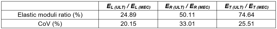
A proportional relation can be seen between the elasticity moduli obtained using both methodologies. Therefore, the values obtained using ultrasound were approximately 25% higher in the longitudinal direction, approximately 50% higher radially, and approximately 75% higher tangentially, than those obtained using mechanical tests. The numerical difference variation coefficients fell within the usual values for wood.

The Poisson’s ratios obtained from every methodology were very similar to each other without much significant statistical difference. Measurements of υ_RL using the mechanical tests were less precise than ultrasound, due to very low strain values.

Table 7 shows the usual relations between elasticity moduli given by Guitard (1987) together with the experimental values obtained from the present research. The difference between the longitudinal elasticity modulus in the grain direction and the radial and tangential moduli was greater than the average for hardwoods. In general, the ratios obtained by ultrasound were found to be closer to the reference values than those obtained by the mechanical tests.

Table 7. Ratios between Elasticity Moduli

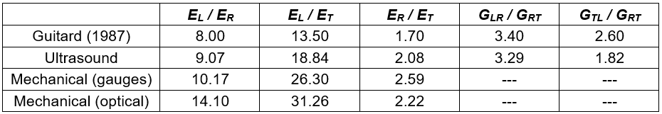
Table 8 shows the experimental values of these relations together with the reference values for hardwoods (Bodig and Jayne 1982).

Table 8. Ratios between Poisson’s Ratio and Elasticity Moduli (Values x10^-5)

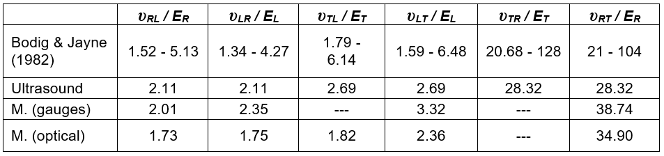
Ultrasound tests perfectly verified the symmetrical ratios because the calculation method itself assumed a priori theoretical orthotropy for the material (C₁₂ = C₂₁, C₁₃ = C₃₁, and C₂₃ = C₃₂). In the mechanical tests using strain gauges, it was only possible to compare the values obtained in the longitudinal and radial directions, with a very small difference between them (2.01 ≈ 2.35), close to the value determined by ultrasound (2.11). Almost symmetrical ratios were also observed in the longitudinal and radial directions from the stereovision measurements asserting the suitability of this procedure. The longitudinal and tangential directions differed in a greater extent. Overall, the ratios obtained by all of the methodologies fell within normal values for hardwoods.

CONCLUSIONS

1. The elastic values of Eucalyptus globulus (Labill.) obtained by ultrasound measurements were higher than those coming from mechanical testing using conventional gauges and the same specimens for both cases. The most noticeable difference between them was found for the longitudinal elasticity moduli.
2. All of the elasticity moduli obtained from stereovision measurements were higher than those that resulted from using conventional gauges. This may lead to the conclusion that local measurements usually provide underestimated values, in comparison to the results from the full-field strain measurements crucial for a non-homogeneous material.
3. The ratios between the different elastic constants fell within the normal reference values for other hardwoods. The results determined by ultrasound were the closest ones, being valid the orthotropic assumptions of the general elastic model.
4. Longitudinal and transversal elasticity moduli indicated that globulus (Labill.) had higher stiffness than that of other hardwoods, making this species of great potential for the development of high added-value products for structural applications. Therefore, the determined elastic constants could be implemented as input parameters in any numerical model.

ACKNOWLEDGMENTS

The results presented were developed within the research project: “Analysis of the stress relaxation in curved members and new joints solutions for timber gridshells made out of Eucalyptus globulus,” BIA2015-64491-P, co-funded by the State Program for the promotion of Scientific and Technical Research of Excellence (2015 call), of the Ministry of Economy and Competitiveness, and European Regional Development Funds (ERDF).

REFERENCES CITED

Aira, J. R., Arriaga, F., and Íñiguez-González, G. (2014). “Determination of the elastic constants of Scots pine (Pinus sylvestris L.) wood by means of compression tests,” Biosystems Engineering 126, 12-22. DOI: 10.1016/j.biosystemseng.2014.07.008

Avril, S., Bonnet, M., Bretelle, A., Hild, F., Ienny, P., Latourte, F., Lemosse, D., Pagano, S., Pagnacco, S., and Pierron, F. (2008). “Overview of identification methods of mechanical parameters based on full-field measurements,” Experimental Mechanics 48(4), 381-402. DOI: 10.1007/s11340-008-9148-y

Bodig, J., and Jayne, B. A. (1982). Mechanics of Wood and Wood Composites, Van Nostrand Reinhold, New York, NY.

Bucur, V. (2006). Acoustics of Wood, Springer-Verlag, Berlin, Germany.

Bucur, V., and Archer, R. R. (1984). “Elastic constants for wood by ultrasonic method,” Wood Science and Technology 18(4), 255-265. DOI: 10.1007/BF00353361

Dahl, K. B., and Malo, K. A. (2009). “Planar strain measurements on wood specimens,” Experimental Mechanics 49(4), 575-586. DOI: 10.1007/s11340-008-9162-0

EN 1912 (2013). “Structural timber- Strength classes- Assignment of visual grades and species,” European Committee for Standardization, Brussels, Belgium.

EN 338 (2010). “Structural timber. Strength classes,” European Committee for Standardization, Brussels, Belgium.

EN 384 (2004). “Structural timber. Determination of characteristic values of mechanical properties and density,” European Committee for Standardization, Brussels, Belgium.

FAIR CT 98-9579 (2001). RTD of Sawmilling Systems Suitable for European Eucalyptus globulus Affected by Growing Stresses, CIS-Madera.

Fernández-Golfín, J. I., Díez, R., Hermoso, E., Baso, C., Casas, J. M., and González, O. (2007). “Caracterización de la madera de Eucalyptus globulus para uso estructural,” Boletín del CIDEU 4: 91-100.

Gibson, L. J., and Ashby, M. F. (2001). Cellular Solids- Structure and Properties, Cambridge University Press, Cambridge, UK.

Gonςalves, J. C., Valle, A. T., and Costa, A. F. (2001). “Estimativas das constantes elásticas da madeira por meio de ondas ultrassonoras (The use of ultrasonic method for estimating wood elastic constants),” Revista Cerne 7(2), 81-92.

Gonςalves, R., Trinca, A. J., and Ferreira, G. C. S. (2011a). “Effect of coupling media on velocity and attenuation of ultrasonic waves in Brazilian wood,” Journal of Wood Science 57(4), 282-287. DOI: 10.1007/s10086-011-1177-y

Gonςalves, R., Trinca, A. J., and Guilherme, D. (2011b). “Comparison of elastic constants of wood determined by ultrasonic wave propagation and static compression testing,” Wood and Fiber Science 43(1), 64-75.

Gonςalves, R., Trinca, A. J., and Pellis, B. P. (2014). “Elastic constants of wood determined by ultrasound using three geometries of specimens,” Wood Science and Technology 48(2), 269-287. DOI: 10.1007/s00226-013-0598-8

Guitard, D. (1987). Mécanique du Matériau Bois et Composites, Cépadues-Editions, Toulouse, France.

Hering, S., Keunecke, D., and Niemz, P. (2012). “Moisture-dependent orthotropic elasticity of beech wood,” Wood Science and Technology 46(5), 927-938.

IFN III (2007). “Third National Forestry Inventory,” Ministry of Agriculture, Feeding, and Environment of Spain, Madrid, Spain.

ISO 3129 (2012). “Sampling methods and general requirements for physical and mechanical testing of small clear wood specimens,” International Organization for Standardization, Geneva, Switzerland.

ISO 13061 (2014). “Physical and mechanical properties of wood, test methods for small clear specimens, and determination of strength in compression perpendicular to grain,” International Organization for Standardization, Geneva, Switzerland.

Lara-Bocanegra, A. J., Majano-Majano, A., Crespo, J., and Guaita, M. (2017). “Finger-jointed Eucalyptus globulus with 1C-PUR adhesive for high performance engineered laminated products,” Construction and Building Materials 135, 529-537.

Majano-Majano, A., Fernandez-Cabo, J. L., Hoheisel, S., and Klein, M. (2012). “A test method for characterizing clear wood using a single specimen,” Experimental Mechanics 52(8), 1079-1096. DOI: 10.1007/s11340-011-9560-6

Mascia, N. T. (2003). “Concerning the elastic orthotropic model applied to wood elastic properties,” Maderas: Ciencia y Tecnología 5(1), 3-19.

Mascia, N. T., and Lahr, F. A. R. (2006). “Remarks on orthotropic elastic models applied to wood,” Materials Research 9(3), 301-310. DOI: 10.1590/S1516-14392006000300010

Ozyhar, T., Hering, S., Sanabria, S. J., and Niemz, P. (2013). “Determining moisture-dependent elastic characteristics of beech wood by means of ultrasonic waves,” Wood Science and Technology 47(2), 329-341. DOI: 10.1007/s00226-012-0499-2

Preziosa, C. (1982). Method for Determining Elastic Constants of Wood by Use of Ultrasound, Ph.D. Thesis, University of Orleans, Orleans, France.

Schmidt, J., and Kaliske, M. (2009). “Models for numerical failure analysis of wooden structures,” Engineering Structures 31(2), 571-579. DOI: 10.1016/j.engstruct.2008.11.001

Sliker, A., Yu, Y., Weigel, T., and Zangh, W. (1994). “Orthotropic elastic constants for eastern hardwood species,” Wood and Fiber Science 26(1), 107-121.

Trinca, A. J., and Gonςalves, R. (2009). “Effect of the transversal section dimensions and transducer frequency on ultrasound dimensions and transducer frequency on ultrasound wave propagation velocity in wood,” Revista Árvore 33(1), 177-184. DOI: 10.1590/S0100-67622009000100019

UNE 56546 (2013). “Clasificación visual de la madera aserrada para uso estructural, Madera de frondosas (Visual grading for structural sawn timber. Hardwood timber),” Madera y Corcho, Spain.

Vázquez, C., Gonςalves, R., Bertoldo, C., Baño, V., Vega, A., Crespo, J., and Guaita, M. (2015). “Determination of the mechanical properties of Castanea sativa (Mill.) using ultrasonic wave propagation and comparison with static compression and bending methods,” Wood Science and Technology 49(3), 607-622. DOI: 10.1007/s00226-015-0719-7

Xavier, J., De Jesus, A. M. P., Morais, J. J. L., and Pinto, J. M. T. (2012). “Stereovision measurements on evaluating the modulus of elasticity of wood by compression tests parallel to the grain,” Construction and Building Materials 26(1), 207-215. DOI: 10.1016/j.conbuildmat.2011.06.012

Article submitted: October 31, 2016; Peer review completed: December 29, 2016; Revised version received and accepted: March 29, 2017; Published:  April 4, 2017.

DOI: 10.15376/biores.12.2.3728-3743