Determination of the most appropriate statistical method for estimating the production values of medium density fiberboard

Abstract

This study determines an optimum method to predict Turkish Medium Density Fiberboard (MDF) production values using ARIMA (Box-Jenkins), regression, and Artificial Neural Network (ANN). The prediction performance of these methods is also compared. A total of 14 independent variables, likely to influence MDF production, were determined, and the production values of the next 9 years (2017-2025) were predicted on the basis of these variables. The test results indicate that the best Mean Squared Error (MSE), Mean Absolute Percentage Error (MAPE), and Mean Absolute Deviation (MAD) prediction performance belongs to the prediction performed with ANN.

Full Article

Determination of the Most Appropriate Statistical Method for Estimating the Production Values of Medium Density Fiberboard

Rifat Kurt

This study determines an optimum method to predict Turkish Medium Density Fiberboard (MDF) production values using ARIMA (Box-Jenkins), regression, and Artificial Neural Network (ANN). The prediction performance of these methods is also compared. A total of 14 independent variables, likely to influence MDF production, were determined, and the production values of the next 9 years (2017-2025) were predicted on the basis of these variables. The test results indicate that the best Mean Squared Error (MSE), Mean Absolute Percentage Error (MAPE), and Mean Absolute Deviation (MAD) prediction performance belongs to the prediction performed with ANN.

Keywords: MDF; ARIMA; Regression; ANN; Prediction

Contact information: Bartin University, Faculty of Forestry, Department of Forest Industry Engineering Bartin, 74100, Turkey; *Corresponding author: rkurt@bartin.edu.tr

INTRODUCTION

Modelling and other prediction methods are widely used in part due to recent developments in technology. Such increased variety of prediction methods has enabled a more thorough evaluation of analyses, thus paving the way for obtaining better results. ARIMA (Box-Jenkins), regression, and Artificial Neural Networks (ANN) are some of the commonly applied prediction methods.

In the literature, these three methods have been widely applied for prediction purposes of fields including production, marketing, finance, stock exchange, agriculture, forestry, food, energy, banking, automotive, and aviation. Many studies have used artificial neural networks (Arizmendi et al. 1993; Fletcher and Goss 1993; Grudnitski and Osburn 1993; Balestrino et al. 1994; Aiken et al. 1995; Kaastra and Boyd 1995; Kiartzis et al. 1995; Gately 1996; Zhang et al. 1998; Kolehmainen et al. 2001; Pijanowski et al. 2002; Huang 2004; Niska et al. 2004; Elminir et al. 2005; Huang 2007; Pindoriya et al. 2008; Hadavandi et al. 2010; Blanco et al. 2012; Miljanović et al. 2017; Bardak 2018; Sozen et al. 2018; Nguyen et al. 2018) and regression analysis (Katipamula et al. 1998; Ghiaus 2006; Wang and Xia 2009; Catalina et al. 2013; Braun et al. 2014; Amiri et al. 2015; Fumo and Rafe Biswas 2015; Sebri 2016; Walter and Sohn 2016; Libaoa et al. 2017).

The ARIMA method has been used in a wide variety of fields as much as the other two methods because of its ease of application (Hamed et al. 1995; Yayar and Karkacier 2003; Altin 2007; Katsoulis and Pnevmatikos 2009; Cenan and Gurcan 2011; Jakaša et al. 2011; Shukla and Jharkharia 2011; Celik 2013; Ayodele et al. 2014; Tavakkoli et al. 2015; Zhang et al.2017). Also, the following papers used at least two of these methods for prediction: Goh (1998); Prybutok et al. (2000); Alon et al. (2001); Ho et al. (2002); Somvanshi et al. (2006); Zou et al. (2007); Koutroumanidis (2009); Sahoo et al. (2009); Zhang et al. (2010); Adebiyi et al. (2014); Ozoh et al. (2014); Voronin and Partanen (2014); Yi et al. (2014); Kaytez et al.(2015); Ertugrul and Bekin (2016); and Hanief et al. (2017).

In this study, the prediction performances of the mentioned methods were compared after prediction of the Medium Density Fiberboard (MDF) production quantities of Turkey.

EXPERIMENTAL

Data

The dependent variable, used in ARIMA, Regression, and ANN models, is the variable that is the subject of the prediction, and it comprises the values related to MDF production in Turkey (Fig. 1). The independent variables to be used in the regression analysis and ANN prediction models were inquired by a team of experts, and 14 variables that were likely to affect MDF production were determined accordingly. These independent variables are: MDF export (m³), MDF import (m³), Furniture export ($), Furniture import($), Consumer Price Index (CPI), Producer Price Index (PPI), Gross National Product Per Capita (GDP), Exchange Rate, Economic Growth (%), Population, Log (m³), Industrial Wood (m³), Building Number, and Building Area (m²). While all of these variables were used in the regression estimation, the number of variables was reduced to ten in order to provide more effective training of the network in ANN estimation. A data set involving a 26-year period (1991-2016) was used for the variables assigned for each product and model. SPSS for regression analysis, MATLAB for artificial neural networks, and MINITAB for ARIMA were used to build the most suitable models for prediction.

Fig. 1. The production amounts of MDF in Turkey (m³) (FAO, 2017)

The future values of the independent variables to be used in the model should also be estimated as a means to make future predictions with regression and ANN models. The estimations for these values for the next nine years (until 2025) were found based on time series, and predictions were made on the basis of these estimated values. Initially, stationarity tests on times series were performed in prediction with ARIMA, and after ensuring stationarity, the most suitable model for prediction was determined. The prediction performances were compared after the calculation of Mean Squared Error (MSE), Mean Absolute Percentage Error (MAPE), and Mean Absolute Deviation (MAD) values, which are widely used in the literature.

ARIMA Method

In cases where time series were stationary, i.e., the average, variance, and covariance of the process varied depending on time, ARMA (p,q) or special versions of this model (AR(p) and MA (q)) were used. However, time-dependent variations in the average and variance of time series could occur in reality. Such situations are called non-stationary states. Such time series can be used after being transformed into stationary states. Stationarizing the time series is possible through evaluating the first and second differences series. In this case, the model is referred to as ARIMA (p,d,q) (Hamzacebi and Kutay 2004; Topcuoglu et al. 2005; Ozdemir and Bahadır 2010).

Introduced by Box and Jenkins, the ARIMA model has been one of the most popular approaches for time series forecasting analysis. The ARIMA model can be used when the time series is stationary and there is no missing data within the time series (Box and Jenkins 1970; Koutroumanidis et al. 2009).

Generally, a nonseasonal time series can be modeled as a combination of past values and errors, which can be denoted as ARIMA (p,d,q) and expressed as a Eq. 1,

 (1)

where  is the actual value,  is the random error at time t,  and  are model parameters, p and q integers that are often referred to as orders of autoregressive and moving average, respectively.

Regression Method

Regression analysis is a statistical procedure that uses the least squares approach in estimating the relationship between independent variables and the dependent variable in developing the estimation model (Cabuk et al. 2011; Cabuk et al. 2014).

If the regression analysis involves one dependent and one independent variable, then it is a simple linear regression. A simple linear regression model is solved with the following equation,

 (2)

where β₀ and β₁ represent the regression coefficients of the model, ε represents the error term, Y represents dependent, and X represents independent variables.

If the regression analysis involves one dependent and two or more independent variables, then it is multiple linear regression. Multiple linear regression models are solved with the following equation,

 (3)

where Y is the dependent variable, X₁,X₂,… X_n are the independent variables, n the number of variables, β₁, β_1… β_n are the regression coefficients, and ε is an error to account for the discrepancy between predicted data and the observed data.

Artificial Neural Network

Artificial neural networks (ANN) are based on the functioning principle of the human brain, and they have emerged as a result of integrating learning processes into computer systems. This model has found a variety of applications ranging from finance and marketing to several engineering sectors. This method has been successful in producing reliable results and effective solutions of complex non-linear problems. For these reasons, this model is commonly used. In this context, ANN are capable of revealing unknown and indiscernible relationships and enabling their effective and optimum use (Kurt et al. 2017).

Artificial neural networks have been proposed as an adaptive evaluation method that can operate with missing data, derive decisions even under uncertain conditions, and tolerate errors (Oztemel 2012). A typical ANN cell is comprised of input data, weights, addition function, activation function, and output (Fig. 2). The data from the outer environment is taken into the ANN through the first layer (input layer). This layer constitutes the parameters that affect the problem. The parameters in the input layer are multiplied by weight coefficients that specify their effect in the neuron, then, the net input received by the neuron is calculated with addition function. Afterwards, this calculated net input value is evaluated by an activation function to determine the corresponding output to be produced. The output value specified by the activation function is then sent to another ANN neuron as input (Kurt et al. 2017).

Fig. 2. A typical artificial neural network cell

The function of the network is described as follows,

 (4)

where Y_j is the output of node j, f is the transfer function, W_ij connection weight between node j and node i in the lower layer, X_ij is the input signal from the node i in the lower layer node j.

RESULTS AND DISCUSSION

Data Analysis, Model Selection, and Forecast

Prior to the prediction process, the data subject to prediction were brought in compliance with each prediction method, and the model was built accordingly.

ARIMA results

The series’ stationarity was checked with “Dickey-Fuller Tests” prior to the prediction process with ARIMA method. Augmented Dickey-Fuller test results are given in Table 1. As indicated by the results, the presence of a unit root is evident as the Dickey-Fuller test statistics of MDF production values exceeded the critical value of 1.836115. Also, the series is not stationary, as the significance (p) level 0.9995>0.05 (Stationarity: If p<0.05, the series is stationary).

Table 1. Augmented Dickey-Fuller Test Results

As also indicated by the declining trend analysis graph, the series is under the effect of seasonal factor (Fig. 3). Dickey-Fuller test results, which were obtained after the evaluation of the second differences of MDF production values, show that the series is completely stationarized and the effect of the seasonal factor is eliminated (Dickey-Fuller test statistics is lower than the critical value of -4.931274, with a significance level of 0.0008<0.05).

Fig. 3a. Trend analysis graphs for MDF production values

Fig. 3b. Trend analysis graphs for MDF production values

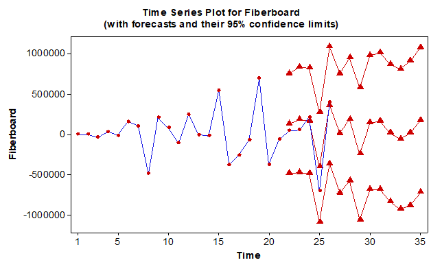
Fig. 4. ARIMA prediction results for 2012-2025 (m³)

After the series was stationarized, different models were applied and as a result of the trials, the ARIMA (5,2,2) model was determined to be the most suitable model for prediction. Upon determination of the best model and statistical validation, the prediction stage was initiated. The prediction results for 2012-2025 period are given in Fig. 4.

Regression results

Dependent and independent variables were entered into the system to determine the most suitable model for prediction, and the best regression model for MDF production was sought accordingly. The regression results, related to the built models are given in Table 2. As shown in the summarized table, all of the regression models built with one variable (Furniture Export), two variables (Furniture Export, Building Areas) and three variables (Furniture Export, Building Areas, CPI) are valid and significant, i.e., they are applicable to the prediction process. In all regression models, coefficients of determination (R²) were found to be significantly high, and the validity of the models were also verified with F statistical values and α=0.05 significance level between dependent and independent variables. In this research, the prediction process was performed with the regression model using three independent variables (Furniture Export, Building Areas, CPI), as the R² =0.989 value represented by three independent variables is a significantly high coefficient of determination. This value indicates that the chosen independent variables predict the MDF production with 98% reliability, thus verifying the suitability of the built linear model.

Table 2. Model Summary and Coefficients

Accordingly, the most suitable regression model for prediction of MDF production can be given with the following expression:

Y_fproduction = -499120.492+ 0.001_Furnexport+0.008_Buildareas+82.955_CPI (model 3)

The t and F statistical test results of the hypotheses that apply for the independent variables and the overall model are given in Table 3.

Table 3. T and F test Results of Independent Variables

Prior to the prediction of MDF production values with the Regression model, the projection of the independent variables for the next nine years were found with ANN with relation to the time series (years) and the projection values were calculated on the basis of these obtained values. The models which were used to predict the independent variables were significant at a level of p<0.05 (Table 4).

Table 4. Regression Equations Used for the Prediction of the Independent Variables

Table 5. Regression Prediction Results for 2012-2025 (m³)

After the determination of independent variables with the best suitable model, the MDF production values for years 2016-2025 were predicted (Table 5).

Artificial neural network results

Ten variables, likely to be effective on the MDF production, constituted the input variables of the ANN model. The feedforward backpropagation ANN was used by the use of input and output neurons. The number of hidden layers was set as 1, and the number of neurons in the hidden layer was set as 8 after a number of trials between 1 and 10. Sigmoid activation function, commonly used for ANN, was used as the activation function. The number of neurons in the output layer was specified as 1, as this value can be equal to the number of dependent variables for cause-and-effect-relation based predictions. The structure of the ANN model, built for MDF production, is given in Fig. 5.

Fig. 5. The structure of the ANN model

Following the determination of the number of input and output neurons for ANN model, independent and dependent variables were subjected to the logarithmic transformation, for ensuring their usability in the system. Twenty-six data sets for each year within the period from 1991-2016 were evaluated, and 70% of these data were used for training, 15% were used for validation, and 15% were used for testing purposes.

For obtaining the optimum results from the model to be built, the number of epochs was kept constant to find the most suitable values for momentum coefficients and learning rate. Trials between 0.1 and 0.9 were made to find the optimum learning rate and momentum coefficients and the most suitable learning rate and momentum coefficients were found as 0.3 and 0.5, respectively.

After the training of the network was completed, testing and validation procedures were performed. For the test of the model, data between 2012 and 2016, which the system has never seen before, were used. Figure 6 shows the change in the error values for the training, validation, and testing sets at each iteration for the MDF production, as well as training status of the network, and regression values. As shown in the figure, regression values are reliable at a rate of about 99% at training, validation, and testing stages.

Fig. 6. Training validation and test results for ANN

After determination of the most suitable coefficients and accomplishing the training of the network, the prediction stage was initialized. Independent variables were predicted and the data were entered into the ANN model to predict the 2016-2025 MDF production values (Table 6).

Table 6. ANN Prediction Results for 2012-2025 (m³)

Comparison of the Prediction Performance

MAD, MAPE, and MSE performance results for MDF production values show that the best performance results were achieved with ANN prediction, which was closely followed by the performance results of the regression prediction results (Table 7).

Table 7. MAD, MAPE, and MSE Performance Results

As indicated by the table, the highest increase in the future MDF production is predicted by ARIMA method, whereas the lowest increase was predicted by ANN. The real and predicted values for all three methods were significantly close for the 2012-2015 period.

CONCLUSIONS

1. A comparative investigation of the prediction performances of ANN, ARIMA, and regression models was performed in the present research. MDF production values until year 2025 were predicted using the 25-year data set for the 1991-2016 period. MSE, MAPE, and MAD performance results for the test data show that the best performance results were achieved by use of the ANN model. The performance of ANN was followed by the Regression and ARIMA models.
2. Considering that some rows in the ANN data set are kept separate for validation and test operations and do not participate in the training, it is seen that they give more accurate results with less data than other estimation methods. Furthermore, the method provided a significant advantage for forecasting as it did not require any preconditions and had a flexible modeling structure.
3. The use of ANN is favored among others especially when the independent values are known. However, the ANN predictions performed with unknown independent variables in the presence of seasonality have been reported to yield low prediction performances. In this regard, independent variables should be chosen to represent the dependent variables in the best possible way, for obtaining the highest prediction performance and precision in future predictions.
4. The regression model, on the other hand, exhibited a close prediction performance to that of ANN, and yielded reasonable results, and thus proved to be an effective method for future predictions. ARIMA method can be an alternative to others, in terms of ease of application time.
5. This study reveals the advantages and disadvantages of three methods (ANN, Regression, and ARIMA) used for future predictions. In this respect, before embarking on a prediction process, a decision maker should take into consideration that the model being built should represent the main case in the best possible way without compromising on time and cost factors. The most suitable model for representation of the existing structure can be achieved, and the best prediction results can be obtained accordingly.
6. The results also will be useful for showing the opportunities and bottlenecks in the forest products sector as well as for the employees and the entrepreneurs in terms of planning, strategy, investment, marketing, raw materials, capacity and demand. The models installed in the project will be updated and used in the production projection calculations of the product mentioned in the following years.

REFERENCES CITED

Adebiyi, A. A., Adewumi, A. O., and Ayo, C. K. (2014). “Comparison of ARIMA and artificial neural networks models for stock price prediction,” Journal of Applied Mathematics 2014, Article ID 614342. DOI: 10.1155/2014/614342

Aiken, M., Krosp, J., Vanjani, M., Govindarajulu, C., and Sexton, R. (1995). “A neural network for predicting total industrial production,” Journal of End User Computing 7(2), 19-23.

Alon, I., Qi, M., and Sadowski, R. J. (2001). “Forecasting aggregate retail sales: a comparison of artificial neural networks and traditional methods,” Journal of Retailing and Consumer Services 8, 147-156. DOI: 10.1016/S0969-6989(00)00011-4

Altin, A. (2007). “Modelling of water amount which goes into Dodurga dam by using Box-Jenkins technique,” Journal of Engineering and Architecture Faculty of Eskisehir Osmangazi University 20(1), 81-100.

Amiri, S. S., Mottahedi, M., and Asadi, S. (2015). “Using multiple regression analysis to develop energy consumption indicators for commercial buildings in the U.S.,” Energy and Buildings 109, 209-216. DOI: 10.1016/j.enbuild.2015.09.073

Arizmendi, C. M., Sanchez, J. R., Ramos, N. E., and Ramos, G. I. (1993). “Time series prediction with neural nets: Application to airborne pollen forecasting,” International Journal of Biometeorology 37(3), 139-144. DOI: 10.1007/BF01212623

Ayodele, A. A., Aderemi, O. A., and Charles, K. A. (2014). “Stock price prediction using the ARIMA model,” 16^th International Conference on Computer Modelling and Simulation, Cambridge, UK, pp. 106-112.

Balestrino, A., Bini Verona, F., and Santanche, M. (1994). “Time series analysis by neural networks: Environmental temperature forecasting,” Automazione e Strumentazione 42(12), 81-87.

Bardak, S. (2018). “Predicting the impacts of various factors on failure load of screw joints for particleboard using artificial neural networks,” BioResources 13(2), 3868-3879. DOI: 10.15376/biores.13.2.3868-3879

Blanco, A. M. Sotto, A., and Castellanos, A. (2012). “Prediction of the amount of wood using neural networks,” Journal of Mathematical Modelling and Algorithms 11(3), 295-307. DOI: 10.1007/s10852-012-9186-4

Box, G. E. P., and Jenkins, G. M. (1970). Time Series Analysis: Forecasting and Control. Holden-Day Inc., San Francisco, CA.

Braun, M. R., Altan, H., and Beck, S. B. M. (2014). “Using regression analysis to predict the future energy consumption of a supermarket in the UK,” Applied Energy 130, 305-313. DOI: 10.1016/j.apenergy.2014.05.062

Cabuk, Y., Karayilmazlar, S., Aytekin, A., and Kurt, R. (2011). “Statistical analysis and projection of wood veneer industry in Turkey: 2007 – 2021,” Scientific Research and Essays 6(13), 3205-3216.

Cabuk, Y., Karayilmazlar, S., Aytekin, A., Onat, S. M., and Kurt, R. (2014). “The Turkish paper and paperboard industry: A Study of the statistical assessment, analysis and forecast,” Journal of the Faculty of Forestry Istanbul University 64(1), 67-69. DOI: 10.17099/jffiu.55245

Catalina, T., Iordache, V., and Caracaleanu, B. (2013). “Multiple regression model for fast prediction of the heating energy demand,” Energy and Buildings 57, 302-312. DOI: 10.1016/j.enbuild.2012.11.010

Celik, S. (2013). “Modelling of production amount of nuts fruit by using Box-Jenkins technique,” Yuzuncu Yıl University Journal of Agricultural Sciences 23(1), 18-30.

Cenan, N., and Gurcan, I. S. (2011). “Forward projection of the number of farm animals of Turkey: ARIMA modeling,” Journal of Turkish Veterinary Medical Society 82(1), 35-42.

Elminir, H. K., Areed, F. F., and Elsayed, T. S. (2005). “Estimation of solar radiation components incident on Helwan site using neural networks,” Solar Energy 79, 270-279. DOI: 10.1016/j.solener.2004.11.006

Ertugrul, I., and Bekin, A. (2016). “Comparative analyses of forecasting models of artificial neural network and time series analyses for selected main food prices in Turkey,” Kafkas University Journal of the Faculty of Economics and Administrative Sciences 7(13), 253-280. DOI:10.9775/kauiibfd.2016.013

Food and Agriculture Organization of the United Nations (FAO) (2017). “FAOSTAT: Food and agriculture data,” (http://www.fao.org/faostat/en/#home), Accessed on 17 April 2017.

Fletcher, D., and Goss, E. (1993). “Forecasting with neural networks: An application using bankruptcy data,” Information and Management 24, 159-167. DOI: 10.1016/0378-7206(93)90064-Z

Fumo, N., and Rafe Biswas, M. A. (2015). “Regression analysis for prediction of residential energy consumption,” Renewable and Sustainable Energy Reviews 47, 332-343. DOI: 10.1016/j.rser.2015.03.035

Gately, E. (1996). Neural Networks for Financial Forecasting, John Wiley, New York.

Ghiaus, C. (2006). “Experimental estimation of building energy performance by robust regression,” Energy and Buildings 38, 582-587. DOI: 10.1016/j.enbuild.2005.08.014

Goh, B. (1998). “Forecasting residential construction demand in Singapore: A comparative study of the accuracy of time series, regression and artificial neural network techniques,” Engineering, Construction and Architectural Management 5(3), 261-275. DOI: 10.1108/eb021080

Grudnitski, G., and Osburn, L. (1993). “Forecasting S and P and gold futures prices: An application of neural networks,” The Journal of Futures Markets 13(6), 631-643. DOI: 10.1002/fut.3990130605

Hadavandi, E., Shavandi, H., and Ghanbari, A. (2010). “Integration of genetic fuzzy systems and artificial neural networks for stock price forecasting,” Knowledge-Based Systems 23, 800-808. DOI: 10.1016/j.knosys.2010.05.004

Hamed, M. M., Al-Masaeid, H. R., and Said, Z. M. B. (1995). “Short-term prediction of traffic volume in urban arterials,” Journal of Transportation Engineering 121(3), 249-254. DOI: 10.1061/(ASCE)0733-947X(1995)121:3(249)

Hamzacebi, C., and Kutay, F. (2004). “Electric consumption forecasting of turkey using artificial neural networks up to year 2010,” Journal of the Faculty of Engineering and Architecture of Gazi University 19(3), 227-233.

Hanief, M., Wani, M. F. and Charoo, M. S. (2017). “Modeling and prediction of cutting forces during the turning of red brass (C23000) using ANN and regression analysis,” Engineering Science and Technology 20(3), 1220-1226. DOI: 10.1016/j.jestch.2016.10.019

Ho, S. L., Xie, M., and Goh, T. N. (2002). “A comparative study of neural network and Box-Jenkins ARIMA modeling in time series prediction,” Computers and Industrıal Engineering42(2-4), 371- 375. DOI: 10.1016/S0360-8352(02)00036-0

Huang, W. (2004). “Forecasting foreign exchange rates with artificial neural networks: A review,” International Journal of Information Technology and Decision Making 3(1), 145-165. DOI: 10.1142/S0219622004000969

Huang, W. (2007). “Neural networks in fınance and economıcs forecastıng,” International Journal of Information Technology and Decision Making 6(1), 113-140. DOI: 10.1142/S021962200700237X

Jakaša, T., Andročec, I., and Sprčić, P. (2011). “Electricity price forecasting – ARIMA model approach,” 8^th International Conference on the European Energy Market (EEM), Zagreb, Croatia, pp. 222-225.

Kaastra, I., and Boyd, M. S. (1995). “Forecasting futures trading volume using neural networks,” The Journal of Futures Markets 15(8), 953-970. DOI: 10.1002/fut.3990150806

Katipamula, S., Reddy, T. A., and Claridge, D. E. (1998). “Multivariate regression modeling,” Journal of Solar Energy Engineering 120(3), 177-184. DOI:10.1115/1.2888067

Katsoulis, B. D., and Pnevmatikos, J. D. (2009). “Statistical analysis of urban air-pollution data in the Athens basin area, Greece,” International Journal of Environment and Pollution36(1-3), 30-43. DOI: 10.1504/IJEP.2009.021815

Kaytez, F., Taplamacioglu, M. C., Cam, E., and Hardalac, F. (2015). “Forecasting electricity consumption: A comparison of regression analysis, neural networks and least squares support vector machines,” Electrical Power and Energy Systems 67, 431-438. DOI: 10.1016/j.ijepes.2014.12.036

Kiartzis, S. J., Bakirtzis, A. G., and Petridis, V. (1995). “Short-term load forecasting using neural networks,” Electric Power Systems Research 33(1), 1-6. DOI: 10.1016/0378-7796(95)00920-D

Kolehmainen, M., Martikainen, H., and Ruuskanen, J. (2001). “Neural networks and periodic components used in air quality forecasting,” Atmospheric Environment 35(5), 815-825. DOI: 10.1016/S1352-2310(00)00385-X

Koutroumanidis, T., Ioannou, K., and Arabatzis, G. (2009). “Predicting fuel wood prices in Greece with the use of ARIMA models, artificial neural networks and a hybrid ARIMA–ANN model,” Energy Policy 37(9), 3627-3634. DOI: 10.1016/j.enpol.2009.04.024

Kurt, R., Karayilmazlar, S., Imren, E., and Cabuk, Y. (2017). “Forecasting by using artificial neural networks: Turkey’s paper-paperboard industry,” Journal of Bartin Faculty of Forestry19(2), 99-106.

Libao, Y., Tingting, Y., Jielian, Z., Guicai, L., Yanfen, L., and Xiaoqian, M. (2017). “Prediction of CO₂ emissions based on multiple linear regression analysis,” Energy Procedia 105, 4222-4228. DOI: 10.1016/j.egypro.2017.03.906

Miljanović, M., Toša, N., Zoran, S., and Tucikesic, S. (2017). “Forecasting geodetic measurements using finite impulse response artificial neural networks,” Indian Journal of Geo-Marine Sciences 46(09), 1743-1750.

Nguyen, T., Nguyen, T., Ji, X., and Guo, M. (2018). “Predicting color change in wood during heat treatment using an artificial neural network model,” BioResources 13(3), 6250-6264. DOI: 10.15376/biores.13.3.6250-6264.

Niska, H., Hiltunen, T., Karppinen, A., Ruuskanen, J., and Kolehmainen, M. (2004). “Evolving the neural network model for forecasting air pollution time series,” Engineering Applications of Artificial Intelligence 17(2), 159-167. DOI: 10.1016/j.engappai.2004.02.002

Ozdemir, M. A., and Bahadır, M. (2010). “Global climate change forecast for Denizli by Using the Box-Jenkins technique,” The Journal of International Social Research 3(12), 352-362.

Ozoh, P., Abd-Rahman, S., and Labadin, J. (2014). “A comparative analysis of techniques for forecasting electricity consumption,” International Journal of Computer Applications 88(15), 8-12. DOI: 10.5120/15426-3841

Oztemel, E. (2012). Artificial Neural Networks. Papatyabilim Publishing, Istanbul.

Pijanowski, B. C., Brown, D. G., Shellito, B. A., and Manik, G. A. (2002). “Using neural networks and GIS to forecast land use changes: A land transformation model,” Computers, Environment and Urban Systems 26(6), 553-575. DOI: 10.1016/S0198-9715(01)00015-1

Pindoriya, N. M., Singh, S. N., and Singh, S. K. (2008). “An adaptive wavelet neural network-based energy, price forecasting in electricity markets,” IEEE Transactıons on Power Systems23(3), 1423-1432. DOI: 10.1109/TPWRS.2008.922251

Prybutok, V. R., Yi, J., and Mitchell, D. (2000). “Comparison of neural network models with ARIMA and regression models for prediction of Houston’s daily maximum ozone concentrations,” European Journal of Operational Research 122(1), 31-40. DOI: 10.1016/S0377-2217(99)00069-7

Sahoo, G. B., Schladow, S. G., and Reuter, J. E. (2009). “Forecasting stream water temperature using regression analysis, artificial neural network, and chaotic non-linear dynamic models,” Journal of Hydrology 378(3-4), 325-342. DOI: 10.1016/j.jhydrol.2009.09.037

Sebri, M. (2016). “Forecasting urban water demand: A meta-regression analysis,” Journal of Environmental Management 183(3), 777-785. DOI: 10.1016/j.jenvman.2016.09.032

Shukla, M., and Jharkharia, S. (2011). “ARIMA models to forecast demand in fresh supply chains,” International Journal of Operational Research 11(1), 1-18. DOI: 10.1504/IJOR.2011.040325

Somvanshi, V. K., Pandey, O. P., Agrawal, P. K., Kalanker, N. V., Prakash, M. R., and Chand, R. (2006). “Modelling and prediction of rainfall using artificial neural network and ARIMA techniques,” Journal of Indian Geophysical Union 10(2), 141-151.

Sozen, E., Bardak, T., Aydemir, D., and Bardak, S. (2018). “Estimation of deformation in nanocomposites using artificial neural networks and deep learning algorithms,” Journal of Bartin Faculty of Forestry 20(2), 223-231.

Tavakkoli, A., Hemmasi, A. H., Talaeipour, M., Bazyar, B., and Tajdini, A. (2015). “Forecasting of particleboard consumption in Iran using univariate time series models,” BioResources10(2), 2032-2043. DOI: 10.15376/biores.10.2.2032-2043

Topcuoglu, K., Pamuk, G., and Ozgurel, M. (2005). “Stochastic modelling of Gediz basin’s precipitation,” Ege Journal of Agricultural Research 42(3), 89-97.

Voronin, S., and Partanen, J, (2014). “Forecasting electricity price and demand using a hybrid approach based on wavelet transform, ARIMA and neural networks,” Internatıonal Journal of Energy Research 38(5), 626-637. DOI: 10.1002/er.3067

Walter, T., and Sohn, M. D. A. (2016). “Regression-based approach to estimating retrofit savings using the building performance database,” Applied Energy 179, 996-1005. DOI: 10.1016/j.apenergy.2016.07.087

Wang, X. W. Q., and Xia, F. (2009). “Integration of grey model and multiple regression model to predict energy consumption,” in: 2009 International Conference on Energy and Environment Technology, Guilin, China, pp. 194-197. DOI: 10.1109/ICEET.2009.53

Yayar, R., and Karakcier, O. (2003). “To determine the model and estimate of future for foreign trade series of agricultural sector (The forecast method of Box-Jenkins),” Journal of Agricultural Faculty of Gaziosmanpasa University 20(2), 89-108.

Yi, X., Jin, X., John, L., and Shouyang, W. A. (2014). “Multiscale modeling approach incorporating ARIMA and ANN’s for financial market volatility forecasting,” Journal of Systems Science and Complexity 27(1), 225-236. DOI: 10.1007/s11424-014-3305-4

Zhang, G., Patuwo, B. E., and Hu, M. Y. (1998). “Forecasting with artificial neural networks: The state of the art,” International Journal of Forecasting 14(1), 35-62. DOI: 10.1016/S0169-2070(97)00044-7

Zhang, G. P., Areekul, P., Member, S., Senjyu, T., Member, S., and Toyama, H. (2010). “A hybrid ARIMA and neural network model for short-term price forecasting in deregulated market,” IEEE Transactions on Power Systems 25(1), 524-530. DOI: 10.1109/TPWRS.2009.2036488

Zhang, K., Gencay, R., and Yazgan, M. E. (2017). “Application of wavelet decomposition in time-series forecasting,” Economics Letters 158, 41-46. DOI: 10.1016/j.econlet.2017.06.010

Zou, H. F., Xia, G. P., Yang, F. T., and Wang, H. Y. (2007). “An investigation and comparison of artificial neural network and time series models for Chinese food grain price forecasting,” Neurocomputing 70(16-18), 2913-2923. DOI: 10.1016/j.neucom.2007.01.009

Article submitted: March 20, 2019; Peer review completed: May 25, 2019; Revised version received and accepted: June 14, 2019; Published: June 19, 2019.

DOI: 10.15376/biores.14.3.6186-6202