Impact of trucking network flow on preferred biorefinery locations in the southern United States

Abstract

The impact of the trucking transportation network flow was modeled for the southern United States. The study addresses a gap in existing research by applying a Bayesian logistic regression and Geographic Information System (GIS) geospatial analysis to predict biorefinery site locations. A one-way trucking cost assuming a 128.8 km (80-mile) haul distance was estimated by the Biomass Site Assessment model. The “median family income,” “timberland annual growth-to-removal ratio,” and “transportation delays” were significant in determining mill location. Transportation delays that directly impacted the costs of trucking are presented. A logistic model with Bayesian inference was used to identify preferred site locations, and locations not preferential for a mill location. The model predicted that higher probability locations for smaller biomass mills (feedstock capacity, the size of sawmills) were in southern Alabama, southern Georgia, southeast Mississippi, southern Virginia, western Louisiana, western Arkansas, and eastern Texas. The higher probability locations for large capacity mills (feedstock capacity, the size for pulp and paper mills) were in southeastern Alabama, southern Georgia, central North Carolina, and the Mississippi Delta regions.

Full Article

Impact of Trucking Network Flow on Preferred Biorefinery Locations in the Southern United States

Timothy M. Young,^a* Lee D. Han,^b James H. Perdue,^c Stephanie R. Hargrove,^d Frank M. Guess,^e Xia Huang,^f Chung-Hao Chen,^g

The impact of the trucking transportation network flow was modeled for the southern United States. The study addresses a gap in existing research by applying a Bayesian logistic regression and Geographic Information System (GIS) geospatial analysis to predict biorefinery site locations. A one-way trucking cost assuming a 128.8 km (80-mile) haul distance was estimated by the Biomass Site Assessment model. The “median family income,” “timberland annual growth-to-removal ratio,” and “transportation delays” were significant in determining mill location. Transportation delays that directly impacted the costs of trucking are presented. A logistic model with Bayesian inference was used to identify preferred site locations, and locations not preferential for a mill location. The model predicted that higher probability locations for smaller biomass mills (feedstock capacity, the size of sawmills) were in southern Alabama, southern Georgia, southeast Mississippi, southern Virginia, western Louisiana, western Arkansas, and eastern Texas. The higher probability locations for large capacity mills (feedstock capacity, the size for pulp and paper mills) were in southeastern Alabama, southern Georgia, central North Carolina, and the Mississippi Delta regions.

Keywords: Biorefinery; Bayesian; Biomass; Transportation; Logistics; Traffic flow; Models; Site locations

Contact information: a: Department of Forestry, Wildlife and Fisheries, Center for Renewable Carbon, The University of Tennessee, Knoxville, TN  37996 USA; b: Civil and Environmental Engineering, The University of Tennessee, Knoxville, TN  37996 USA; c: USDA Forest Service, Southern Research Station, Knoxville, TN  37996 USA; d: Civil and Environmental Engineering, The University of Tennessee, Knoxville, TN  37996 USA; e: Department of Statistics, Operations, and Management Science, The University of Tennessee, Knoxville, TN  37996 USA; f: Center for Renewable Carbon, The University of Tennessee, Knoxville, TN  37996 USA; g: Department of Electrical and Computer Engineering, Old Dominion University, Norfolk, VA 23529 USA; *Corresponding author: tmyoung1@uk.edu

INTRODUCTION

As noted in the Billion-Ton Report (Langholtz et al. 2016), feedstock economic availability will be influenced by delivered costs, which may be greatly dependent on transportation costs. This Billion-Ton Report notes the need for more research on delivered costs at the plant-gate, which is directly addressed in this research study.

As noted in several studies, the freight truck transportation infrastructure must adapt to an expanded presence of domestic biofuels production, which implies understanding and reducing congestion delays that result annually in 11 million tons of CO₂  production (Biomass Research and Development Board 2008, Myers and Slone 2010). These constraints increase trucking costs and are problematic to the emerging bioeconomy.

This research studies the impacts of transportation infrastructure and related risk for the emerging bioeconomy. Regions with major truck freight were modeled for increased flow and contrasted with regions without comparable flow rates. Bayesian priors were developed from the network flow models for these regions to estimate posterior distributions for probabilistic-based prediction.  Bayesian methods were used in this study given the improvements in sensitivity and specificity in validation relative to other methods.  This is discussed in more detail in the manuscript. This study uses accepted GIS-based methodologies and geospatial modeling integrated with Bayesian statistical methods to site optimal locations for biorefineries (see the helpful text by Eksioglu et al. (2015) on GIS methods and biorefinery site location).

Estimating the availability of woody biomass for bioenergy and biofuel production has been the subject of much research (see as an example, Perez-Verdin et al. 2009; Munsell and Fox 2010; Welfle et al. 2014).  There are many other noteworthy works that would be too extensive to list in a manuscript. These previous works established the theoretical framework for using such data with other relevant data to develop geospatial analyses for siting biorefineries.  The motivation for this research builds upon these previous studies to develop statistical-based models for determining preferred locations for biorefineries.  Given this rationale, the research study had the following objectives.

Objectives and Scope

There were four study objectives.  The first objective was to identify zones in the southern U.S. that are probable locations for the emerging bioeconomy in the presence of high transportation flow. The second objective was to assess the current transportation flow for these regions and model the impact of increased truck transportation flow for select types of bioenergy feedstocks.  The third objective was to estimate the transportation costs in the selected regions and compare such costs with other potential bioeconomy regions that do not have transportation flow bottlenecks.  These first three objectives address one of the questions noted by the Biomass Research and Development Board (2008), whereas as mentioned above, the need for studying future growth of biofuels on the transportation network is identified as a key research requirement. The fourth objective was to develop Bayesian prior and posterior distributions for transportation flow times for the above regions and identify optimal site locations for biorefineries (Young et al. 2011; Huang et al. 2012). The fourth objective satisfies a gap in the research, where there are no publications in the public domain that have used Bayesian inference and traffic flow to estimate probabilistic locations for biorefineries with traffic flow adjusted transportation costs. The study region consisted of the states of Alabama, Arkansas, Florida, Georgia, Kentucky, Louisiana, Mississippi, North Carolina, Oklahoma, South Carolina, Tennessee, Texas, and Virginia.

EXPERIMENTAL

Materials

Transportation network simulation flow model software

Multiple meetings were held with Dr. Samuel Jackson of Genera Energy, LLC at the Vonore, TN biofuel plant, and operational information and traffic volumes were acquired for existing and projected commercial facilities.  Dr. Jackson has expertise in the start-up of a new biorefinery and has strong knowledge of the influence of transportation flows on actual delivered transportation costs.  His knowledge of the transportation flows within a non-concentric procurement zone proved invaluable to validating study results. Farm-routing information was imported into Google Earth for projecting actual traffic flow of switchgrass (Panicum virgatum) feedstock supply. Switchgrass trucks in the Vonore, TN area were followed to study their routes and potential height, weight, and width concerns that need to be considered in the traffic modeling effort. Traffic modeling tools were compared including TransCAD (Caliper Corp., Newton, MA, USA), Synchro/SimTraffic (Trafficware Inc., Sugarland, TX, USA), and MATSim (Senozon Deutschland GmbH, Berlin, Germany). It was decided to use Synchro for the modeling task (OptTek Systems, Inc. 2005). A Synchro/SimTraffic model for the vicinity of Vonore, TN and the road network and signal- timing was developed.

A microscopic simulation study, using realistic traffic patterns, was designed to examine the effects that a new biofuel plant may have on its surrounding roadway network (Hwang et al. 2006; Chin et al. 2009). This was valuable for considering the siting of such a plant, e.g., rural versus urban locations, and determining its adverse traffic impacts (Han et al. 2003, 2007). Multiple existing plant sites were examined, and the biofuel plant in Vonore, TN was chosen. The plant provides a good representation of typical biofuel plant sites in terms of its roadway network, operational information, and traffic volumes.

Vonore is a small town with a population of 1,474 with 1,172 potential drivers. The town has experienced a steady population growth of about 27% in the past decade. The town has a total area of less than 12 square-miles and is situated along the bank at the confluence of the Little Tennessee River and Tellico River. A map of the roadway network near Vonore and the biofuel plant is shown in Fig. 1. The main road through Vonore is US Route 411 (US 411), a four-lane roadway with a median and two shoulders. This road connects the Town of Vonore northeasterly to Knoxville and southwesterly to Madisonville. Tennessee State Route 72 (SR 72), a two-lane road, connects the town to Interstate 75 (I-75) to the north. State Route 360 (SR 360), another two-lane road, connects the town to many rural areas to the south. The town has become an ideal site for many warehouses and factories, including Home Depot, because of its proximity to Knoxville and convenient access to the highway, railway, and waterway.

The historical traffic demand data for the Vonore area were extracted from the Tennessee Department of Transportation (TDOT) Annual Average Daily Traffic (AADT) data book for the years 1985 through 2012. The vehicle distribution was determined by field observation during peak hours. In Fig. 2, the local AADTs and peak hour volumes (PHV), for both directions are provided for major roadways. The AADTs for smaller roads were unavailable.

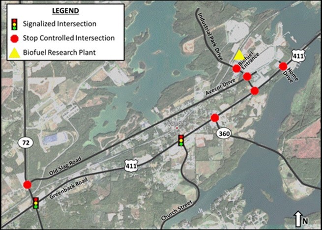
Fig. 1. Map of Vonore, TN 

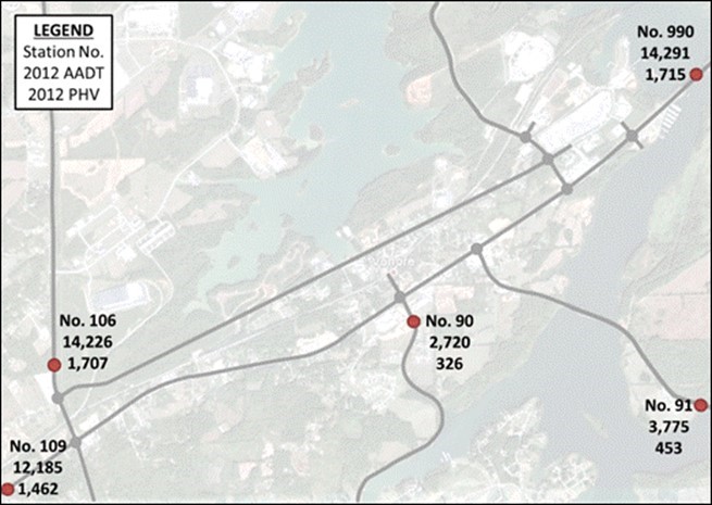
Fig. 2.  Local AADT and PHV for Vonore, TN

When simulating the local traffic based on the 2012 traffic demand, the existing biofuel research facility is included in the volumes. To evaluate the largest effect that the biofuel plant could have on a roadway network, the morning (AM) and evening (PM) peaks were examined. The existing AM and PM peak volumes were generated for the whole roadway network (black lines in Fig. 1), using the observed turning movement counts and the peak hour volumes that were 12% of the 2012 AADT (Fig. 2).

To simulate various levels of biofuel plant traffic, Dr. Jackson was consulted to determine the plant’s operational level and traffic volumes for existing and projected plant activities. Farm-to-plant switchgrass truck routing information was also acquired and imported into Google Earth maps for the purpose of a real-world trip assignment of switchgrass trucks. To determine the optimal and/or shortest paths for switchgrass trucks, field visits were conducted in the Vonore area to study the routes used by switchgrass trucks and their potential height, weight, and width concerns that were reflected in the traffic modeling effort.

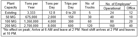
The biofuel plant in Vonore processes just over 3,000 tons of material annually. The switchgrass trucks do not operate on a daily basis at the facility, but it is common to have 20 switchgrass deliveries in one day, using 5 trucks. To model the trip generation of switchgrass trucks for much larger commercial biofuel plants, scenarios with production levels ranging from 50, 100, to 200 million gallons (MG) per year were studied. Table 1 summarizes the trip generation anticipated for the existing research plant and potential commercial facilities. To determine the number of trucks needed for each factory, it was assumed that each truck had a maximum capacity of 20 tons with a 0.7 load factor to capture all of the partially loaded trucks. For example, a 50 MG plant requires 2,000 tons of switchgrass per day. However, a 20-ton truck with the 0.7 load factor applied will only carry 14 tons each trip, thus requiring 142.8 deliveries per day. For the simulation the number was rounded to 150 deliveries per day for the 50 MG plant to yield a conservative estimation of the trip generation. The employee trips were not included in any simulation because the trips were expected to occur at shift change times, 6:00 am, 2:00 pm, and 10:00 pm, outside of the peak periods.

 Table 1. Biofuel Facilities Trip Generation

Truck traffic distribution was estimated for the biofuel plant as follows:

• North   SR 72              46%
• West    US 411            42%
• East     US 411            12%

Figure 3 illustrates the anticipated traffic assignment of the trucks on the existing street network. The distribution was determined by using the existing farm-routing information and shortest path calculations.

Evaluating the current operations of the traffic control devices, capacity, and Level of Service (LOS) were calculated using methods from the 2000 Highway Capacity Manual, Special Report 209 (Transportation Research Board 1999). Signalized and un-signalized intersections were evaluated based on estimated intersection delays.

Fig. 3. Truck trip distribution in for biofuel facilities

The LOS and capacity are the measurements of an intersection’s ability to accommodate traffic demand. The LOS for intersections ranges from A to F, where an LOS of A is best, and an LOS of F is failing. For signalized intersections, a LOS of A has an average estimated intersection delay of less than 10 s, and an LOS of F has an estimated delay of greater than 80 s per vehicle. An LOS of C and D are typical design values. With urban areas, an LOS of D, which is a delay between 35 s and 55 s, is considered acceptable by the Institute of Transportation Engineers (ITE) for signalized intersections.

The LOS at un-signalized intersections has lower thresholds of delay. An LOS of F exceeds a delay of 50 seconds. For urban arterials, minor approaches may frequently experience an LOS of E. A full LOS description for signalized and un-signalized intersections is given in the report by the Transportation Research Board (1999).

Delay, LOS, and capacity analyses were conducted using the Synchro 7 software (Trafficware Inc., Sugarland, TX) developed by Trafficware. Seven scenarios were designed and analyzed for the peak hour. The first four were of different facility sizes (existing, 50 MG, 100 MG, and 200 MG) with the current 2012 peak hour volumes. The last three assume a moderate 100 MG facility with the 2012 peak hour volumes experiencing a growth of 5%, 15%, and 50%. If Vonore continues its current rate of growth, these rates would be comparative of the next two, six, and 20 years, respectively.

For each simulated scenario, the traffic signal timing plans were optimized, and the signal offset was appropriately configured. This level of optimization is atypical of the real-world practice, which tends to be less efficient. While it is common to retime traffic signals in the surrounding network when a commercial facility is constructed, it is rare that the updated traffic signal timing plans are optimized.

The realistic commercial biofuel plant capacity for a town like Vonore is 100 MG; therefore, multiple scenarios for the AM peak period with a 100 MG facility were studied.  Figure 4 shows the LOS at various locations with the existing research facility, while Fig. 5 shows the LOS with a 100 MG facility in year 2012. The circles at the center of each intersection represent the LOS, while the colored lines represent the LOS of each roadway segment approaching the intersection.

To emulate the effect of a growing population in the vicinity of Vonore, a growth rate was applied to the existing 2012 volumes. The construction of a commercial-grade biofuel plant not only generates additional trips to-and-from the facility, but also causes additional population and possible business growth. Figures 6 and 7 present the anticipated impacts of a 15% and 50% growth from the 2012 volumes on the LOS values. Both figures have undesirable LOS F situations at many of the intersections and approaches along State Route 72 and US Route 411. The figures also illustrate that the Industrial Park Drive is expected to experience minimal change with the population growth, but this could change with the addition of more commercial facilities.

From the transportation network analysis, it was clear that the actual day-to-day trips of a biofuel facility had minimal influence on the Vonore roadway network. What remains unseen is the effect of the biofuel trucks on the low-volume roads that surround the farms.

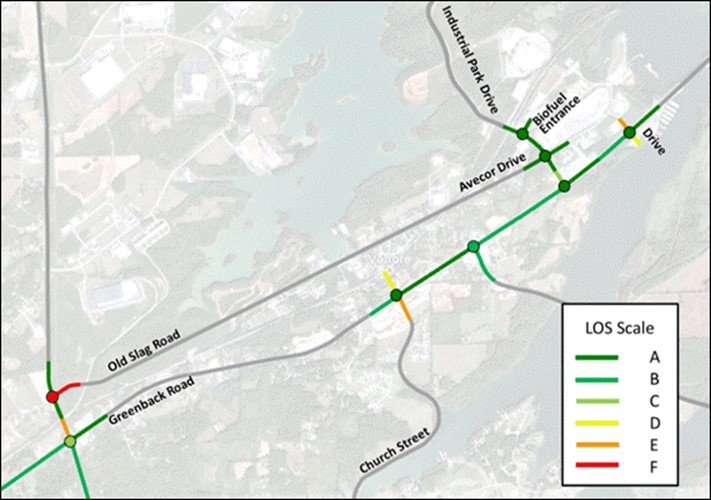
Fig. 4. LOS of 2012 AM peak traffic with existing research facility

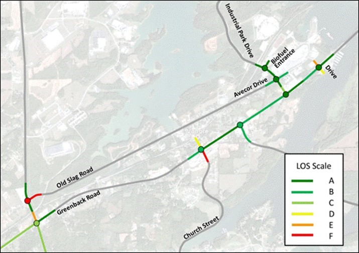
Fig. 5. LOS of 100 MG facility with 2012 AM peak traffic

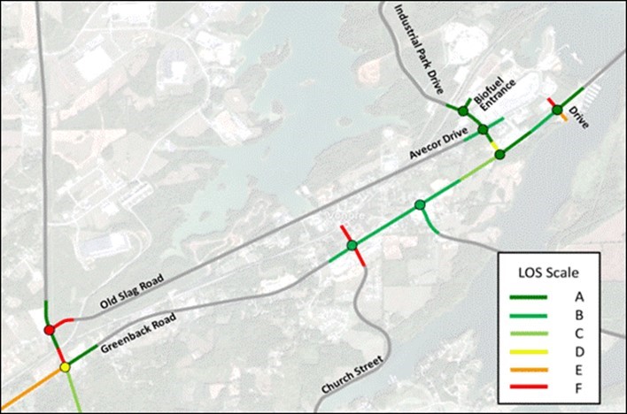
Fig. 6. LOS of 100 MG facility with 2012 AM peak traffic grown 15%

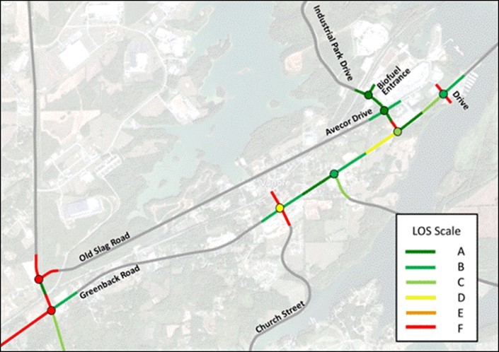
Fig. 7. LOS of 100 MG facility with 2012 AM peak traffic grown 50%

Databases and study group

Using the National Renewable Energy Laboratory (2009) definition, “bioenergy and biofuel plants are facilities that integrate woody biomass conversion processes, and equipment to produce wood pellets for energy, biofuels, biopower, or value-added biochemical,” 60 such facilities were known to exist in the study area. Given the fact that many of ZCTAs do not contain bioenergy mills (which is a problem for logistic regression) wood-using facilities were used as substitutes (e.g., sawmills, oriented strand board or OSB mills, and pulp and paper mills). As a number of authors have noted, similar geo-spatial and economic factors may influence site preference given the commonality of the feedstock procurement systems (Moon et al. 2008; Knight 2009; Cohen et al. 2010; Patari 2010).

            Group I:  Sawmills illustrated in Fig. 8.

Group II: Pulp and paper, OSB, and wood pellet mills illustrated in Fig. 9.

Response and Explanatory Variables

There were two response variables. For Group I, the variable, y_­­i1 = 1 if i^th ZCTA had at least one woody biomass-using facility, and y_­­i2 = 1 for Group II mills (Fig. 8 and Fig. 9). Fourteen predictor variables from the public domain data were examined in the relational database for further statistical analyses (Table 2).

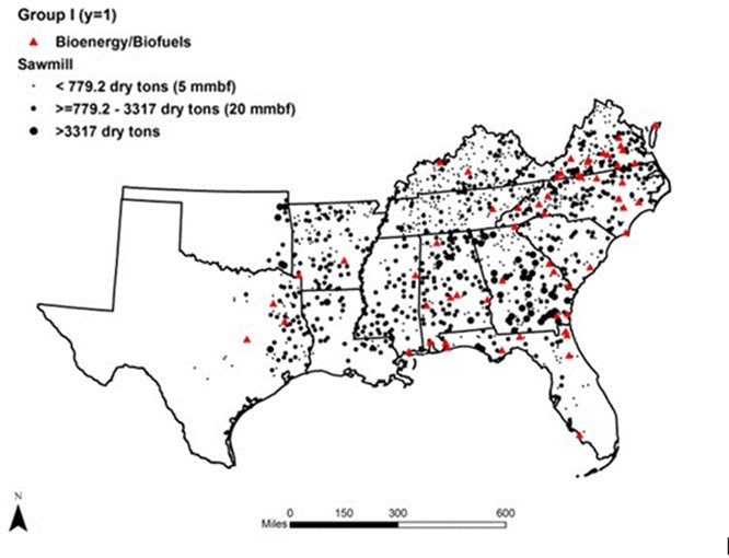
Fig. 8. Illustration of Group I woody biomass-using mills

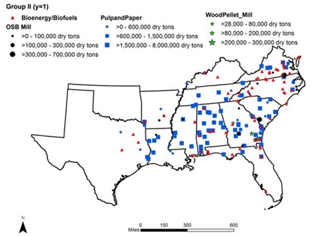
Fig. 9. Illustration of Group II woody biomass-using mills

The explanatory variables in the study were selected based on the prior research of Young et al. (2011) and the ability to create a complete geo-spatial relational database from databases that exist in the public domain.  Prior research by Wear et al. (2007) suggested that population and household densities and associated incomes, as well as farm income level, have an influence on determining the amount of forestland in non-urban or non-suburb productive use, i.e., less land available in productive forestland affects procurement zones and delivers raw material costs.  Other variables such as forestland ratio, urban land ratio, crop cultivated land ratio, and timberland growth-to-removal ratio also influence the amount of forestland in productive use and costs of delivered fiber.  Road density and transportation delays influence transportations costs.  The number of primary processing mills can act in positive synergy for larger pulp mill size biorefineries that use the residual feedstocks for raw materials, while the number of primary processing mills typical of smaller capacity sawmill type mills may act as a negative competitive influence on site location of a smaller biorefinery. 

Table 2. Explanatory Variables Organized by ZCTA

METHODS

Logistic Regression Model for Siting Biorefineries

Large volumes of data were organized into a relational database from the U.S. Census Bureau (2010a; 2010b), U.S. Forest Service (2009), U.S. National Land Cover Database (2006), U.S. National Elevation Dataset (2010), U.S. Department of Agriculture National Agricultural Statistic Service (2008), U.S. Environmental Protection Agency (2011), and from BioSAT (Perdue et al. 2011). BioSAT provides geo-spatially implicit information on economic biomass quantity (Zalesny et al. 2016).

BioSAT was used to estimate the woody biomass supply for procurement zones assuming a 128.8 km one-way hauling distance given the existing road network. The supply from restricted areas was not considered in the estimates (e.g., national parks, national forests, urban areas, etc.). See Huang et al. (2012) for more detail on the geo-spatial road networks used in the study. Data were compiled at the U.S. Census Bureau 5-digit ZIP Code Tabulation Area (ZCTA) level. There were 10,016 ZCTAs (average area of 209.84 km) in the study region that represented the potential sites for woody biomass plants.

Logistic Regression

The logistic regression methodology was inspired by Young et al. (2011). This study applied the Bayesian inference for estimation of the parameters in the logistic regression models. The Bayesian inference specifies the probability distribution for the underlying categorical or continuous variables and estimates parameters β (see Eqs. 1 and 2). Bayesian inference allows for incorporation of prior beliefs and the combination of such beliefs with statistical data that are well suited for representing the uncertainties in the value of independent variables (Hilborn et al. 1994). For example, by expressing the uncertainties in parameter vector β for a model M as the posterior probability distribution p(β│M,D), where D are the observed data, see Eqs. 1 and 2,

        (1)

where,

                     (2)

The key of Bayesian inference is to choose the parametric family for the prior probability distributions. Two categories were used: non-informative prior distributions and informative prior distributions. A non-informative prior distribution expresses general information about a parameter. A common non-informative prior distribution is the uniform distribution and always yields similar results as classical statistics. Thus, Bayesian and classical statistics are not exclusive; rather they are overlapped to some extent. In fact, classical approaches are approximately Bayesian using certain priors. An informative prior distribution reflects specific and definite information about a parameter. If both prior and posterior distributions are the same, the prior distribution is called a “conjugate prior distribution,” which is a case in informative prior distributions. In this study two prior distributions were selected from non-informative and informative prior distributions and were constructed on parameter b, according to Eqs. 3 and 4,

                                        (3)

                   (4)

The statistical software package WinBUGS^® (Windows Bayesian Inference Using Gibbs Sampling) (MRC Biostatistics Unit, Cambridge, UK) was used for the Bayesian inference analysis. It provided a convenient environment to conduct a Markov Chain Monte Carlo simulation (MCMC) of parameters β, which converges to a stationary joint distribution. In each analysis, one independent chain was run for 10,000 iterations. Convergence was assessed by visual inspection and by the Gelman et al. (2000) shrink factor. The ZCTA-level data were partitioned into two parts using a stratified random sampling technique for each state which ensured a spatially proportionate data allocation across the study region: 80% for training and 20% for validation. The training data were used to develop the models while the validation data were used to test model performance.  The general schema of the methodology is presented in Fig. 10.

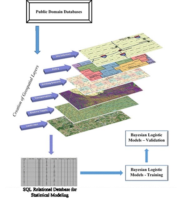
Fig. 10. Illustration of the general schema of methodology 

Results and Discussion 

Trucking Costs and Delay Times

The delay times for each state were estimated from the study using the Synchro and SimTraffic models. Average trucking costs ($/dry ton) were estimated using the trucking cost model of BioSAT. The descriptive statistics of the trucking costs from the BioSAT model are given in Table 2. Average trucking costs varied from $15.52/dry-ton to $17.34/dry-ton across the study region. The coefficient of variation for these trucking costs varied from 5.09% in SC to 30.59% in FL and TN.

The costs associated with transportation delay times for trucks were derived from Gillett (2011). Average delay minutes per state varied from 1.12 minutes in OK to 17.93 minutes in TN (Table 3). Delay times had significant influences on the trucking costs by state. Delay times have the potential to increase trucking costs by as much as 61% in certain states within the study region. Recall the statistical significance of transportation delays in the Bayesian logistic regression models determining site location.

Table 3. Descriptive Statistics of Trucking Costs ($/dry ton) by State as Estimated from the BioSAT Model

Table 4. Statistical Interval of Trucking Costs ($/dry ton) by State Adjusted for Average Delay Time per State

Group I

Five out of the possible 14 predictor variables were statistically significant (p-value < 0.05) from the stepwise logistic regression (Table 5).  To compare the MLE and Bayesian inference estimation methods for parameter coefficients, the classification tables are displayed in Tables 4 and 5.  The classification tables confirmed that the logistic regression with Bayesian Inference had good predictive power for Group I facilities (Tables 6 and 7).

Table 5. Significant Variables for Group I Mills

Table 6. Summary of Classification Table for Training Dataset for Group I Mills

Table 7. Summary of Classification Table for Validation Dataset for Group I Mills

The sensitivity of this model assuming a uniform prior in validation was 89% (e.g., predicts a mill location correctly-), and specificity was 92.3% (e.g., predicts the absence of mill correctly) (Tables 6 and 7). The sensitivity rates were higher than 75% of the stringent criteria required for medical screening (Carney et al. 2010).

“Median family income,” “timberland annual growth-to-removal ratio,” and “transportation delays” were highly significant in influencing the mill location (p-values < 0.0001, Table 3). Other significant variables were urban land area ratio, and water area ratio. A higher family income and larger urban area had negative coefficients (Table 3), which suggested that urban developed areas were not suitable for siting mills. The results are in agreement with other studies, i.e., that mill locations were closer to the rural biomass supply. Timberland annual growth-to-removal ratio and water area ratio had positive coefficients. This indicated that landscape with abundant forestland and water areas were preferred. Transportation delays had a positive coefficient, which showed that the mill location may have significant impacts on the local transportation networks. These results suggest the importance of landscape suitability and woody biomass availability on mill location and mill location influence on the adjoining transportation system.

Four ordinal levels for ranking the estimated probability from the logistic model (Bayesian Inference with a uniform prior) in the study region are illustrated in Fig. 11. The higher probability locations for Group I mills were clustered in the southern Alabama, southern Georgia, southeast Mississippi, southern Virginia, western Louisiana, western Arkansas, and eastern Texas regions.

Fig. 11. Estimated probability locations for Group I

Group II

Five out of 14 predictor variables were statistically significant (p-values < 0.05) from the stepwise logistic regression (Table 8). The classification tables confirmed that the logistic regression with Bayesian inference had good predictive power for Group II for the model using Bayesian Inference assuming a uniform Bayesian prior distribution (i.e., equal probabilities of occurrence) having a sensitivity of 88.1% and specificity of 89.2% for Group II training data (Table 9). The sensitivity of this model was 90.5% and specificity was 87.7% (Table 10). The logistic model for Group II was a suitable prediction model for preferred and non-preferred locations. 

Table 8. Significant Variables for Group II Mills

Table 9. Summary of Classification Table for Training Dataset for Group II Mills

Table 10. Summary of Classification Table for Validation Dataset for Group II Mills

Median family income, urban land area ratio, number of primary wood processing mills in each ZCTA, and transportation delays were significant in determining mill location with p-values < 0.0001 (Table 8). The water area ratio was also significant. The median family income had negative coefficients in the model. The urban land area ratio, water area ratio, number of primary wood processing mills in each ZCTA, and transportation delays had positive coefficients in the model. This finding confirms that the local transportation system impacts Group II facilities.

Four-levels for ranking the estimated probability from the logistic model (Bayesian Inference with a uniform prior) are illustrated in Fig. 12. The higher probability locations for Group II mills were clustered in the southeast Alabama, southern Georgia, central North Carolina, and Mississippi Delta regions.

With any research study, it is important to consider the shortcomings of the research for future research considerations.  The challenge of science in the context of statistical inference is obtaining high quality data.  A challenge in geo-spatial analysis is the requirement of high quality data that are ‘complete,’ from which data overlays can be developed to further develop a relational database that is required for statistical models, such as the Bayesian logistic model developed in this study.  The development of a relational database from public domain sources was a non-trivial component of the research that required sufficient resources and scientist-hours.  Future research needs to address the research of ‘data quality’ for geospatial analyses.  Future research also needs to address updating databases of existing mill locations and capacities which are necessary for validation of model results.

Fig. 12. Estimated probability locations for Group II

CONCLUSIONS

The analysis of mill locations for the emerging bioeconomy using Bayesian logistic regression in the presence of trucking delays had several important outcomes.

1. Transportation delays for trucks were statistically significant in influencing site location of bioenergy plants.
2. Transportation delays can strongly impact trucking costs for biomass.
3. The Bayesian logistic model adequately predicted preferred and non-preferred sites.
4. The higher probability locations for larger biomass using mills were clustered in southeast Alabama, southern Georgia, central North Carolina, and the Mississippi Delta regions.
5. The higher probability locations for smaller biomass mills were clustered in southern Alabama, southern Georgia, southeast Mississippi, southern Virginia, west Louisiana, west Arkansas, and east Texas regions.

ACKNOWLEDGMENTS

The authors are grateful for the support of this research provided in part by a grant from the Southeastern Sun Grant Center with funds provided by the U.S. Department of Transportation Research and Innovative Technology Administration. Support for this research was also provided in part by The University of Tennessee, Center for Renewable Carbon, Department of Civil Engineering, Department of Forestry Wildlife and Fisheries, and U.S. Forest Service, Southern Research Station. The authors also thank Dr. Samuel Jackson, Vice President, Genera Energy, LLC.

REFERENCES CITED

Biomass Research and Development Board (2008). “National biofuels action plan,” U.S. Department of Agriculture and U.S. Department of Energy, pp. 24, (www.usda.gov/documents/NBAP081208.pdf), Accessed on date 01/27/2017

Chin, S., Hwang H., Peterson, B. E., Han, L. D., and Chin, C. (2009). “Routing hazardous materials around the District of Columbia area,” J. Transp. Safety Secur. 1(4), 296-313. DOI: 10.1080/19439960903412571

Cohen, J., Janssen, V., and Stuart, P. (2010). “Critical analysis of emerging forest biorefinery (FBR) technologies for ethanol production,” Pulp. Pap.-Canada (1), 24-30.

Eksioglu, S. D., Panos, S. R., and Pardalos, P. (2015). Handbook of Bioenergy, Bioenergy Supply Chain – Models and Applications, Springer International, Switzerland.

Gelman, A., Carlin, J. B., Stern, H. S., and Rubin, D. B. (2000). Bayesian Data Analysis, Chapman & Hall, London, UK.

Gillett, J. C. (2011). Monetizing Truck Freight and the Cost of Delay for Major Truck Routes in Georgia, Master’s Thesis, Georgia Institute of Technology, Atlanta, GA.

Han, L. D., Chin, S., and Hwang, H. (2003). “Estimating adverse weather impacts on major US highway network,” in: TRB Annual Meeting Compendium of Papers, No. 03-2155. DOI: 10.3141/2121-13

Han, L. D., Yuan, F., and Urbanik II, T.  (2007). “What is an effective evacuation operation,” J. Urban Plan D-ASCE 133(1), 3-8. DOI: 10.1061/(ASCE)0733-9488(2007)133:1(3)

Hilborn, R., Pikitch, E., and McAllister, M. (1994). “A Bayesian estimation and decision analysis for an age-structured model using biomass survey data,” Fish. Res. 19(1-2), 17-30. DOI: 10.1016/0165-7836(94)90012-4

Huang, X., Perdue, J. H., and Young, T.M.  (2012). “A spatial index for identifying          opportunity zones for woody cellulosic conversion facilities,” Int. J. For. Res. 2012:1-11.  DOI:10.1155/2012/106474

Hwang, H., Chin, S., Han, L. D., and Yuan, F. (2006). “Synthesizing truck origin-destination table for local transportation analysis zones: A Nashville metropolitan area case study,” Transportation Research Circular E-C088, pp. 145-148, (http://onlinepubs.trb.org…nepubs/circulars/ec088.pdf), Accessed on 01/26/2017.

Knight, D. K. (2009). Wood Bioenergy, Hatton-Brown Publishers, Inc., Montgomery, AL.  DOI: 10.3141/2121-13

Langholtz, M. H., Stokes, B. J., and Eaton, L. M. (2016). 2016 Billion-ton Report: Advancing Domestic Resources for a Thriving Bioeconomy, Volume 1: Economic Availability of Feedstock, Oak Ridge National Laboratory, Oak Ridge, Tennessee, managed by UT-Battelle, LLC for the U.S. Department of Energy.  DOI: 10.1089/ind.2016.29051.doe

Moon, E., Saveyn, B., Proost, S., and Hermy, M. (2008). “Optimal location of new forests in a suburban region,” J. Forest Econ. 14(1), 5-27.  DOI: 10.1016/j.jfe.2006.12.002

Munsell, J. F., and Fox, T. R. (2010). “An analysis of the feasibility for increasing woody biomass production from pine plantations in the southern United States,” Biomass Bioenerg. 34(12), 1631-1642 DOI: 10.1016/j.biombioe.2010.05.009

Myers, D. and Slone, S.  (2010). Green Freight Transportation, Council of State Governors, (http://knowledgecenter.csg.org/drupal/system/files/CR_GreenFreight.pdf), Accessed on 04/24/2017. (http://knowledgecenter.csg.org/drupal/system/files/CR_GreenFreight.pdf), Accessed on 01/26/2017.

National Renewable Energy Laboratory. (2009). “What is biorefinery?” [Biorefinery definition], Retrieved from http://www.nrel.gov/biomass/biorefinery.html. Accessed on 01/26/2017.

OptTek Systems, Inc. (2005). ‘OptQuest® optimization software package,” http://www.opttek.com/. Accessed on 01/26/2017

Perez-Verdin, G, Grebner, D. L., Sun, C., Munn, I. A., Schultz, E. B., and Matney, T. G. (2009). “Woody biomass availability for bioethanol conversion in Mississippi,” Biomass Bioenerg. 33, 492-503 DOI: 10.1016/j.biombioe.2008.08.021

Patari, S. (2010). “Industry-and company-level factors influencing the development of the forest energy business – insights from a delphi study,” Technol. Forecast Soc. (77), 94-109.  DOI: 10.1016/j.techfore.2009.06.2004.

Perdue, J. H., Young, T. M., and Rials, T. G. (2011). “The Biomass Site Assessment Model – BioSAT,” Final Report for U.S. Forest Service, Southern Research Station submitted by the University of Tennessee, Knoxville, 282. http://www.srs.fs.usda.gov/pubs/45655. Accessed on 01/26/2017

Transportation Research Board. (1999). “Final Report – NCHRP 3-55(2) A Planning Applications for the Year 2000 Highway Capacity Manual,” 2101 Constitution Avenue, Washington, D.C. 20418.  http://onlinepubs.trb.org/onlinepubs/archive/NotesDocs/finrep.pdf. Accessed on 01/26/2017

U.S. Census Bureau. (2010(a)). “2010 Census ZIP code tabulation areas” [Data file], Retrieved from http://www.census.gov/geo/reference/zctas.html. Accessed on 01/26/2017

U.S. Census Bureau. (2010(b)). “2010 Urban and rural classification” [Data file], Retrieved from http://www.census.gov/geo/reference/urban-rural.html. Accessed on 01/26/2017

US Department of Agriculture, Forest Service (2015). “Forest and inventory national database 3.0.,” http://www.fia.fs.fed.us/tools-data/.  Accessed on 01/26/2017

U.S. Department of Agriculture National Agricultural Statistics Service.  (2008). “Census of agriculture: farm net income” [Data file], Retrieved from http://www.nass.usda.gov/#top. Accessed on 01/26/2017 http://energy.gov/eere/bioenergy/2016-billion-ton-report Accessed on 01/26/2017

U.S. Environmental Protection Agency.  (2011). “Ecoregions of the United States” [Data file], Retrieved from https://developer.epa.gov/u-s-level-iii-and-iv-ecoregions-u-s-epa-2/.. Accessed on 01/26/2017

U.S. Forest Service. (2009). “Lands in public preserves” [Data file], Personal contact on   08/2011

U.S. National Elevation Dataset.  (2010). “National elevation dataset 1 arc second” [Data file], Retrieved from https://catalog.data.gov/dataset/national-elevation-dataset-ned-1-arc-second-collection. . Accessed on 01/26/2017

U.S. National Land Cover Database.  (2006). “Multi-resolution land characteristics consortium” [Data file], Retrieved from http://www.mrlc.gov/nlcd2006.php. Accessed on 01/26/2017Wear, D. N., Carter, D. R., and Prestemon, J.  (2007).  “The U.S. South’s timber sector in 2005: a prospective analysis of recent change,” Gen. Tech. Rep. SRS–99, Asheville, NC, U.S. Department of Agriculture Forest Service, Southern Research Station

Welfle, A., Gilbert, P., Thornley, P. (2014). “Increasing biomass resource availability through supply chain analysis,” Biomass Bioenerg. 70, 249-266 DOI: 10.1016/j.biombioe.2014.08.001

Young, T. M., Zaretski, R. L., Perdue, J. H., Guess, F. M., and Liu, X. (2011). “Logistic regression models of factors influencing the location of bioenergy and biofuels plants,” BioResources 6(1), 329-343. DOI: 10.15376/biores.6.1.329-343

Zalesny, R. S., Stanturf, J. A., Gardiner, E. S., Perdue, J. H., Young, T. M., Coyle, D. R., Headlee, W. L., Banuelos, G. S., and Hass, A. (2016).  “Ecosystem services of woody crop production systems,” BioEnergy Res 9(2), 465-491. DOI:10.1007/s12155-016-9737-z

Article submitted: January 6, 2017; Peer review completed: March 26, 2017; Revised version received and accepted: April 28, 2017; Published: May 15, 2017.

DOI: 10.15376/biores.12.3.4754-4775