Investigation of biomass char gasification kinetic parameters using a novel miniaturized educational system

Abstract

A novel miniaturized, transparent reactor system for use as either a research or educational tool was developed for investigating biomass char gasification with oxygen to determine the kinetic parameters. Parametric temperature and pressure data taken can be used to distinguish the validity of assumptions inherent in the Avrami, the random pore (RPM), the unreacted core shrinking (UCSM), and a UCSM hybrid models (HM). The results demonstrate the UCSM for spherical and cylindrical geometries, and an HM variation with a best-fit exponent, that yields residual sums of squares 2 to 4 orders of magnitude lower than other models. An Arrhenius evaluation yielded an activation energy of 84.8 kJ/mol and pre-exponential factor of 1.34  103 s-1. An O2 reaction order of 0.85 indicates O2 adsorption on the char surface is the primary rate-controlling step. Data are consistent with a rapidly decreasing surface area as the reaction nears completion, suggesting available corresponding active sites for rapid chemisorption decrease as the reaction progresses. More importantly, the design of the system is safe to take into the classroom while simultaneously allowing students to view real-time reactions and produce repeatable data; this pushes the bounds on classroom interventions and learning.

Full Article

Investigation of Biomass Char Gasification Kinetic Parameters Using a Novel Miniaturized Educational System

Jacqueline K. Gartner,^a Manuel Garcia-Perez,^b and Bernard J. Van Wie ^c,*

A novel miniaturized, transparent reactor system for use as either a research or educational tool was developed for investigating biomass char gasification with oxygen to determine the kinetic parameters. Parametric temperature and pressure data taken can be used to distinguish the validity of assumptions inherent in the Avrami, the random pore (RPM), the unreacted core shrinking (UCSM), and a UCSM hybrid models (HM). The results demonstrate the UCSM for spherical and cylindrical geometries, and an HM variation with a best-fit exponent, that yields residual sums of squares 2 to 4 orders of magnitude lower than other models. An Arrhenius evaluation yielded an activation energy of 84.8 kJ/mol and pre-exponential factor of 1.34 10³ s^-1. An O₂ reaction order of 0.85 indicates O₂ adsorption on the char surface is the primary rate-controlling step. Data are consistent with a rapidly decreasing surface area as the reaction nears completion, suggesting available corresponding active sites for rapid chemisorption decrease as the reaction progresses. More importantly, the design of the system is safe to take into the classroom while simultaneously allowing students to view real-time reactions and produce repeatable data; this pushes the bounds on classroom interventions and learning.

Keywords: Gasification; Biomass conversion kinetics; Unreacted core shrinking model; Hybrid model; Educational system; Biochar

Contact information: a: School of Engineering, Campbell University, Buies Creek, NC, 27506-0115 USA; b: Biological Systems Engineering, Washington State University, Pullman, WA,991644-6120 USA; c: The Gene and Linda Voiland School of Chemical Engineering and Bioengineering, Washington State University, Pullman, WA, 99164-6515, USA; * Corresponding author: bvanwie@wsu.edu

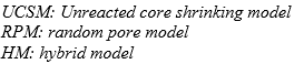
Acronym List

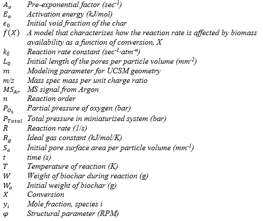
Variable List

INTRODUCTION

The abundance and renewability of biomass make it a candidate for satisfying society’s needs to maintain energy security and reliability (Turner 1999). One attraction is that biomass is carbon neutral (Spliethoff and Hein 1998), which further mitigates concerns about release of greenhouse gases from energy production. Currently, renewable energy has a 14% share in US energy products, which is lower than coal (30%) and natural gas (34%), with biomass occupying only 1.5% of the total picture (US Energy Information Association 2017). Clearly, there is opportunity for growth in renewables, especially biomass, to increase in market share especially in production of synthesis gas (mainly CO and H₂) as it can be upgraded via Fischer-Tropsch synthesis into long chain hydrocarbons for production of fuels like gasoline, diesel, and jet fuel (Chum and Overend 2001). Training a workforce with a clear understanding of the gasification process is critical to catalyzing the implementation of this technology.

To enhance workforce preparedness in the gasification arena, trainees need to understand the technical barriers to be able to determine kinetic rates, and to understand reaction mechanisms so that better biomass conversion processes can be developed. Several technical barriers remain in advancing biomass conversion processes for production of syngas such as scaling and commercializing reactors (Wyman 1999; Perlack et al. 2005) and mass transfer between gas and liquid phases (Wang et al. 2008). Other needs relate to understanding the significant variability in measurements obtained for kinetic parameters that depend on biomass structure and composition, especially inorganic content (Dupont et al. 2015), reactor geometry and mode of operation, methods of sample preparation, oxidation agents used, and biomass mineral content (Senneca 2007; Dupont et al. 2011). Variation between types of wood and activation energies exist, as shown by Di Blasi’s (2009) investigation of soft pine that revealed kinetics determined using a temperature ramp of 10 K/min yielded an activation energy of 125 kJ/mol. Comparatively, Liu et al. (2015) investigated the differences in soft bituminous coal blended with hardwood, and at a heating rate of 10 K/min found an activation energy of 112.4 kJ/mol for a 20% hardwood/80% coal blend, and a lower activation energy of 80.7 kJ/mol for 100% hardwood samples. At a heating rate of 90 K/min the activation energy for the 20/80 blend was 99.4 kJ/mol and for hardwood 55.7 kJ/mol. Beyond experimental conditions, model selection, rate-controlling mechanisms, and reaction order are also important factors to consider. The reaction order when using O₂ as the gasification agent varies widely. Kashiwagi and Nambu (1992), using cellulose powder, report an overall order of 0.78 using 0.28% to 21% by volume O₂; Luo and Stanmore (1992) using sugarcane bagasse report an order of 0.65 with 0% to 21% O₂ by volume; and Varhegyi et al. (2006) using corncob report a reaction order of 0.53 using 21% volume O₂. To isolate the effect of wood type, Fung and Kim (1990) used a shrinking core model on coal and wood, showing that coal gasification is surface reaction controlled while wood is ash layer diffusion controlled. Prestipino et al. (2018) investigated steam gasification of agricultural chars, finding reaction orders ranging between 0.4 and 1 (2018). These findings offer insight into the mechanism that controls the overall reaction. However, with such variability, investigation of both experimental and modeling factors is critical for a complete understanding of these processes.

Robust instruments exist for determining kinetic parameters; however, there are limitations. Thermogravimetric analysis, differential scanning calorimetry, and gas chromatography systems approaches that provide real time data are time consuming and prohibitive for classroom use. Needed is the demonstration of a simple system that can be used reliably and safely in the classroom or by students new to a research group, especially given the challenges presented for graduate and undergraduate students in understanding chemical kinetics (Freeman et al. 2013).

In this study a low-cost experimental apparatus is presented, consisting of an easy to assemble quartz micro-reactor for biochar gasification. The reactor is heated by a resistance wire, sparsely wrapped to enable viewing, surrounded by a see-through borosilicate thermal insulation shield with reflective coating to reduce radiative heat losses, but which can retain a non-silvered viewing window. The micro-reactor by virtue of its size produces a relatively small amount of thermal energy. It is powered by an accompanying voltage supply, all of which may be surrounded by a plexiglass case to shield observers from hot componentry and protect from release of pressurized gases, though such an event is unlikely given the design and operating instructions. To demonstrate the efficacy of the system for the provision of reaction rate data, testing kinetic hypotheses, and acquiring kinetic parameters, temporal syngas production using on-line mass spectrometry (MS) was monitored, making the system useful as an ancillary lab exercise suitable for advanced graduate or undergraduate students in determining global kinetics. Reaction rate data may be extracted from recorded product gas molar flow rates, and kinetics determined by runs at varied temperatures and O₂ partial pressure yielding a pre-exponential factor, Arrhenius activation energy, and reaction order. The experimental results, including conversion vs. time, reaction rate vs. conversion for determining reaction order, selection of the most appropriate reaction process model, determining of kinetic parameters, and the fundamental mechanisms that would support the results obtained are discussed.

METHODS AND MATERIALS

This section begins with a review of gas solid kinetic relationships and modeling used to inform data collection and analyses in light of reaction mechanisms. It continues with a description of the apparatus and instrumentation, followed by a safety emphasis, and then experimental and analysis procedures.

Gas-solid Reactions

Gas-solid reactions are important to model because of the numerous applications, including interest in the combustion and gasification of coal or biomass more generally (Burnham 2017). In this case it is important to show that the new reactor system can serve as an instructional tool for discriminating fundamental reaction behavior as supported by goodness of fit of various models with experimental data. When considering the modeling of these reactions, they are assumed to be non-catalytic. It is also assumed that the interface between the gas and solid moves as the reaction progresses. The general form for the rate of biomass conversion for a gas-solid reaction as defined in the literature (Laurendeau 1978; Fung and Kim 1990; Di Blasi 2009) appears in Eq. 1, with the typical Arrhenius temperature dependency (Khawam and Flanagan 2006), shown in Eq. 2 and the expression for conversion in Eq. 3,

where X is conversion of a solid particle, is the initial weight (g), W is the weight at any time as the reaction proceeds (g), and  is the final weight (g), which in the case considered is assumed to be 0 because the char contains 98.4% carbon, 1.24% hydrogen, and the balance nitrogen,  the activation energy (kJ/mol),  the pre-exponential factor (sec^-1), R the universal gas constant (J/g/° C), T the temperature (K), and  the O₂ partial pressure raised to a reaction order. The function  represents a model that characterizes how the reaction rate is affected by biomass availability as conversion, X, continues toward reaction completion. From a fundamental mechanistic viewpoint, gasification reactions occur via active sites on the char surface (Lin et al. 1991; Woodruff and Weimer 2013; Zhou et al. 2017), per Eqs. 4 through 6, which show the major products CO and CO₂ from a gasification process.

Equation 4 shows the chemisorption of O₂ on the surface of two active sites, whereas Eqs. 5 and 6 show the formation of CO and CO₂ associated with desorption, and the surface reaction combined with desorption, respectively. In these cases we are considering a kinetic expression that globally represents a set of reactions that initiate with carbon and O₂ and complete with the formation of CO, through a series of adsorption and desorption steps (Tseng and Edgar 1985; Hurt and Calo 2001). Given the assumptions of 1) a homogenous surface, with a uniform distribution of active sites, no interaction among adsorbed species, and either nonexistent, or very rapid surface migration; and 2) reaction, so only adsorption or desorption can be rate-controlling, the resulting O₂ reaction order for CO formation can be argued to be either zero or first-order depending on the pressure and the temperature (Hayward and Trapnell 1964; Frank-Kamenetskii 1969). These two extremes can be defined by considering the ratio of the rate of adsorption to the rate of desorption, , (Hayward and Trapnell 1964) multiplied by the concentration of the gasification agent, in this case O₂. If this value is significantly lower than 1, near 0, desorption is fast, adsorption rates control the kinetics, and the reaction order will be near 1. If, however, adsorption is very fast relative to desorption, then is greater than 1, desorption is rate controlling, and the reaction order is near 0. Obviously, the reactant concentration, or the partial pressure, is a significant factor, as is the activation temperature. Adsorption controls at reactant partial pressures in the 0 to 0.21 range, because there are fewer collisions of O₂ molecules with the carbon surface, i.e., mass action effects are limiting. At higher activation temperatures, the surface of the char is converted from micropores to macropores, which results in a reduction in molecular sieve structures, increasing the availability of active sites for adsorption (Laurendeau 1978). At higher concentrations and lower temperatures, however, desorption is rate-controlling because an abundance of O₂ immediately fills the available active sites (Hayward and Trapnell 1964; Frank-Kamenetskii 1969). However, a significant range of O₂ orders have been reported in the literature varying from 0.53 to 0.87 (Luo and Stanmore 1992; Cozzani 2000; Di Blasi 2009) and are attributed to competition between the adsorption and desorption reactions. The take home message is the partial pressure of O₂ is an important consideration and needed for modeling efforts (Kashiwagi and Nambu 1992), and the experimentally determined dependency on O₂ partial pressure offers insights into reaction mechanisms (Laurendeau 1978; Janse et al. 1998; Ye et al. 1998; Zhang et al. 2006). It is notable that ½ order dependency is predicted by adsorption with dissociation as pointed out by both Hayward and Trapnell (1964) and Frank-Kamenetskii (1969), which results in an important caveat, i.e., given different assumptions of chemisorption, desorption, and surface migration, the global expression and rate dependency with respect to heterogeneous kinetics will change. In these applications, CO was the species of interest for modeling as it is desired as a definitive gasification product. In addition, it forms at relatively high concentrations in test runs, thus providing substantive data from which model parameters can be obtained.

Because the reactor was operated at higher temperatures, it is initially assumed that the surface adsorption of O₂ is rate limiting or at least a major contributor to the control of the reaction rate if a reaction order of less than 1.0 is found. To begin the analysis, four gas-solid particle reaction models were considered, all of which describe the surface reaction. These include a classical nucleation model whereby the reacting interface including binding sites is spread evenly throughout the porous solid. A variation of this is the RPM, which includes a pore parameter, allowing for changing surface area with increasing pore diameter initially followed by pore coalescence as conversion increases, a feature not captured by the other models considered. In addition, a model for the reaction interface being on the surface of a nonporous shrinking solid particle was considered. Finally, a derivative of the shrinking model with an adjustable exponent was employed that when fitted to the data offers insight into the geometrical influences on biomass availability.

Modeling

Avrami model

First is the homogenous model (Molina and Mondragón 1998; Bhat et al. 2001), also called the volume reaction model (Bhatia and Perlmutter 1980), or the uniform conversion model (Ye et al. 1998) in gasification kinetics literature. Its true origins are from circa 1940, and it was developed by Kolmogorov (1937), Johnson and Mehl (1939), and Avrami (1939), all of whom independently developed the model. It is a nucleation model that describes how a solid particle transforms uniformly via growth, consumption, or crystallization, and it has since been applied to chemical kinetics (Burnham 2017). The kinetic application assumes that the reaction becomes initiated uniformly throughout the unconverted volume, within the pores and on the surface, and continues until the entire volume is reacted. The model is named after its originators, often taking on a number of letters depending on how many are given credit, and has been called the Avrami model, especially among chemical engineers, the JMA or JMAK (Burnham 2017) equation and the Mampel model (Prasannan et al. 1986); it is shown as Eq. 7.

f(x) = (1 – X) (7)

This rate law is used to describe the differential change in volume. A necessary assumption is that of changing the particle density over time (Burnham 2017), which allows for modeling of the consumption of the solid mass as the reaction progresses while keeping the volume constant. The reaction occurs on all surfaces throughout the volume, with the total mass decreasing uniformly and the reaction rate decreasing linearly with conversion.

Random pore model

The second model in this study is the random pore model (RPM), developed by Bhatia and Perlmutter (1980), which includes a term for structural changes in the porous solid over time. The model includes a solid with a series of pores or cylinders where the reaction occurs uniformly across all surfaces. However, because of pore and surface area changes, the reaction rate can increase as pore diameter increases, but then it can decrease as pores enclose or overlap as they coalesce over time. The model is shown in Eq. 8 and an expression to describe the heterogeneity of the solid and the initial pore structure is shown in Eq. 9,

where  is the initial pore structure parameter, a dimensionless value;  is the initial length of the pores per particle volume (mm^-2);  is the initial void fraction of the char, and  is the initial pore surface area per particle volume (mm^-1).

If  , then Eq. 5 reduces to the Avrami model, highlighting that the Avrami model represents a uniformly porous volume but does not capture the heterogeneity of the structure and the coalescence of the pores during the reaction, a phenomenon described by the contribution of  .

Unreacted core shrinking model

The third model is the unreacted core shrinking model (UCSM), also referred to as the shrinking core model originally proposed in the 1950s by Yagi and Kunii (1955), and in the 1970s it was paired to gasification (Szekely and Evans 1970; Szekely and Evans 1971; Sohn and Szekely 1972). The modeling starts with solid biomass that shrinks as the reaction progresses until the reactants are completely depleted and the residual ash is all that remains. For all but flat slabs the surface area changes with time, which could affect the reaction rate, especially if the surface reaction is the controlling resistance. However, because of the density difference between the solid and reacting gases, core shrinkage is slower by about 1,000 times (roughly the density ratio of solids to gases) than the flow rate of O₂ into the core and a pseudo steady state is assumed in the model derivation (Doraiswamy and Uner 2013). The resulting reaction rate is derived by considering a series of resistances that represent the diffusion of the gas to the surface of the solid, e.g., the prospective diffusion through an ash layer depending on the molecular content of the biomass, the chemical reaction at the gas-solid interface, the diffusion back through the ash layer, and the diffusion back to the bulk fluid. A critical assumption with these resistances is a nonporous solid, assuming the reaction occurs only at the gas-solid interface. In gasification, the chemical resistance is typically the controlling factor (Molina and Mondragón 1998), and whether an ash layer forms or the particle simply shrinks in size as the char is consumed is immaterial from a modeling standpoint. Equation 10 is the general form of the conversion-time relationship for a shrinking core or shrinking particle where differing values of m result during model derivations (Zhang et al. 2010). For a flat plate m = 0, for spheres m = 2/3, and for a cylinder m = ½.

Processes may be shifted to conditions in which the chemical reaction is the controlling factor by minimizing reactant concentration. Verification is accomplished by fitting experimental data with a chemical reaction control form of a model such as in the work by Bhat et al. (2001), where they investigated rice husk char gasification.

Hybrid model

Because of the complexity of the char gasification process, often times neither the Avrami, RPM, nor the UCSM models sufficiently describe the results. Thus, an alternative hybrid model (HM) approach is taken, leaving the exponent in Eq. 10 as an unknown and it is determined empirically in a data fitting process. Investigators report a variety of values from 0.48 to 1 for a range of biomass sources (Zhang et al. 2014), with explanations for the varying exponent that include linking the mechanism to the controlling resistance in the case of the UCSM or describing the first order dependence by making a case for a homogenous reaction mechanism in the case of the Avrami model. Of course, the determination of m can also be used to confirm the control of the chemical reaction in a uniform reaction throughout the biomass, or for a shrinking core situation for a known geometry or it can account for unconventional geometries (Xiang et al. 2002; Shuai et al. 2013). This could be of particular importance in this study as a very small piece of biochar was used in the 4 mg range, which then rests on the lower surface of a cylindrical reactor such that not all sides are equally exposed to the gas phase.

Reactor Assembly and Instrumentation

The experimental apparatus shown in Fig. 1a consists of a quartz reactor that is 10 cm long with a 3-mm OD, 2-mm ID (Technical Glass Products, Painesville, OH), and wrapped with a 20-cm long Kanthal A-1 resistance wire (EZ Cloudz, London, UK), connectors, a power source, resistance wire, and fittings for gas tight flow, with components for one end shown in Fig. 1b. For experiments, a small ~4 mg piece of biochar from the stock shown in Fig. 1c was placed into the quartz reactor and the resistance wire was attached to an HY1803DL 18V 3A linear DC variable power supply (Mastech, San Jose, CA) via alligator clips. Attached to the reactor were ¼” brass tee fittings (McMaster-Carr, Santa Fe Springs, CA) with the two perpendicular legs attached to gas inlet and outlet flow, and straight run legs were attached to a 1/8” converter fitting for the thermocouple wire entrance and exit sealed with silicone O-rings to prevent gas leakage. Thermocouple wires were joined as a butt-weld type K thermocouple (Omega, Norwalk, CT) and placed at the reactor center. A 12-mm OD, 11-mm ID borosilicate tube surrounded the reactor and was held in place by smaller diameter rings on the two end fittings. The inside of this tube facing the reactor was entirely coated with an adhesive silvered tape acting as a radiation shield to reduce heat loss and thereby increase the reactor temperature. Resistance wires exited small grooves cut into the two opposite ends of the borosilicate shield.

Fig. 1. a) Schematic of reactor setup. The quartz reactor was wrapped with a resistance wire and surrounded by a silvered borosilicate shield. Three-way fittings on the ends allowed gas flow in or out, and provided thermocouple exits; b) One end of reactor was setup with fittings, o-rings, reactor, and resistance wire; c) Sample of biochar stock used in each reaction – only a small ~4 mg piece of this biochar was actually used in a given experiment

Safety Emphasis

Safety has been a critical concern in the experimental design and proposed classroom system. The experiments were performed in a hood, and the small ~4 mg of biochar contained a low amount of energy in the reactor, such that if all the biochar instantaneously reacted a small volume of syngas, < 15 mL, would be released and vented from the fume hood. In case the inner tube did crack from built-up pressure, the outer annular tube, as well as the hood, would protect the user from injury. For classroom use, more extensive safety precautions were incorporated such as a plexiglass viewing box that prevents students from touching the hot reaction shield. This further prevents hazards from glass shards should the system be inadvertently over pressurized, though even that is unlikely due to the small amount of biochar loaded into the quartz micro-capillary tube, and the fact that the plastic tubing from the gas loading syringe tubes is more likely to fail before the glass. Further safety issues are discussed in companion work that fully describes the range of uses for the system, including pyrolysis and combustion (Gartner 2018).

Experimental Procedure

The biochar in Fig. 1c was produced from a birch toothpick, a hardwood, by placing it under N₂ for 60 min at 750 °C. A carbon, hydrogen, nitrogen (CHN) test was performed, yielding an elemental analysis with 98.4% C, 1.24% H, 0.14% N, and a sum total of 0.22% other elements. In each run, approximately 4 mg of sample was placed into the reactor, with glass wool on either end to ensure the biochar stayed within the wrapped resistance wire section to ensure constant temperature. Figure 2 shows the entire system setup with the reactor attached to an inlet cylinder containing a mixed stream of 10% O₂ and 90% Ar. A flowmeter was used to regulate the flow of the inlet stream. Prior to placement of biochar in the reactor, experiments were performed to establish base temperature conditions. Five power supply voltages were used, 12 V, 13.4 V, 14.2 V, 16 V, and 17.8 V, a feed stream of 10% O₂ and 90% N₂ supplied at 7.1 ml/min, and the reactor was surrounded by a 100% silvered reflective borosilicate radiation shield to prevent convective and radiative energy losses (Graviet et al. 2015). These settings correspond to baseline temperatures of 650 °C, 700 °C, 750 °C, 800 °C, and 850 °C which were then used to determine reaction rates for model discrimination and determining the Arrhenius parameters.

Fig. 2. Reactor and analysis system. The reactor has a resistance wire attached to a DC power source with a concentric silvered radiation and convection shield to minimize loss of thermal energy and maintain process temperatures as monitored with a type K thermocouple through the center. The inlet flow comes from a cylinder and the outlet flow goes to an MS. An Ar backpressure was applied before the inlet to the MS to prevent diffusion of air into the MS as it pulls a vacuum that can create a low-pressure region especially for streams with very low flow rates.

For reaction order studies, the inlet flow of O₂ was created by combining flows from a cylinder of pure Ar and a separate O₂ cylinder at metered flowrates to attain 0.021 bar, 0.047 bar, 0.068 bar, and 0.10 bar O₂ partial pressures. In all cases, outlet streams were analyzed by connecting to an Inficon Transpector® CPM 2.5 Compact Process Monitor online mass spectrometer (MS) (Syracuse, NY, USA) for continuous monitoring at a rate of one sample every two seconds. The MS was calibrated to detect masses of 2, 15, 18, 28, 44 corresponding to known concentrations of the gasification products, i.e., H_2, CH₄, H₂O, CO, CO₂, as well as 40 and 32 for the carrier gas Ar and unconverted feed O₂ , respectively. The mass number of 15 for CH₄ was chosen because a calibratable portion was ionized and detectable as CH₃⁺ in the MS; this is necessary because ions with a mass of 16 also represent atomic oxygen species created during MS ionization of CO₂ or O₂. Also, the CO signal at 28 was artificially high because of the ionization of CO₂. To account for the increase, 10% of the 44 m/z value for CO₂was subtracted from the CO value, as prescribed by the manufacturer’s fracking data. The reaction was monitored until completion, when CO signals were within 3σ of baseline MS average readings for this species before commencement of the reaction. This time point aligned with O₂ signals, which were within 3σ of average MS readings for final steady state O₂levels. A stream of Ar was added at a flow rate of 1 mL/min to the reactor exit flow with the final flowrate measured to account for concentration changes. The Ar stream was added because the MS operates by pulling a vacuum to receive samples and because of low feed rates to this miniature reactor an increase in flow of the exit stream prevents entrance and back diffusion of air through fittings just prior to the MS. Exit MS baseline signals were used to verify that the exit gas indeed consisted of only Ar and 10% O₂, adjusted for the 1 ml/min add-in stream, before turning on the heating element to initiate gasification to ensure there were no significant air leaks in the system. The Ar signal and flow rate were also used to determine the molar flow rate of all other monitored species.

Data Analysis

Converting MS signals to species molar flow rates began with a calibration for both Ar and O₂, as shown in Eq. 11,

where  is the signal from the MS for Ar,  is the mole fraction of Ar in the stream, and  is the total pressure in the system. Sensitivity coefficients were determined for Ar and O₂. Ar was detected using a mass number of 40, and three concentrations of 5% O₂ / 95% Ar, 10% O₂ / 90% Ar, and 20% O₂ / 80% Ar were run for initial calibration.

To get individual calibrations of species of interest, Ar was combined with H₂ with an m/z of 2 and 2%, 3.5%, and 5% mole fractions; CO, with an m/z of 28 and 2%, 5%, and 10% mole fractions; CO₂ with an m/z of 44 and 2%, 5%, and 10% mole fractions; CH₄ with an m/z of 15 and 2%, 5%, and 8% mole fractions; and H₂O with an m/z of 18 and 2%, 5%, and 10% mole fractions. These were used to establish a linear calibration for each gas species. The formula for partial pressures is shown in Eq. 12,

where  is the mass spec voltage readings for species i and  is the background mass spec voltage reading. The background is an average of 50 time points taken once every two seconds for 100 s before the experiment began,  and  are the ratio of the sensitivity coefficient ratio for species i to that of Ar, and the sensitivity coefficient for Ar values, respectively, from calibrations. Partial pressures were converted into mole fractions using the ideal gas law, and mole fractions multiplied by the total flow to determine species molar flow rates. The limit of detection for the MS itself is 1.1 10^-9, the range of which was prescribed by the manufacturer, and confirmed during calibrations, and a signal for any curve recorded below this threshold was reported as a zero reading. A representative run appears in Fig. 3, from which further analysis strategy is explained. The baseline O₂ up to 165 s represents the non-reacting system exit gases, besides Ar, before the power to the resistance wire was provided. Between 227 s and 300 s the reactor temperature rapidly rose to 700 C, promoting a spike in pyrolysis CO (see small CO spike at the bottom of the graph at 239 s) typically associated with a temperature rise for carbonaceous biomass (Fagbemi et al. 2001; Demirbaş 2002). The corresponding spike in O₂ represents a non-steady state flush of unreacted O₂ out the reactor exit due to the rapid formation of pyrolysis CO and other non-monitored higher MW species, and a sudden increase in temperature, which increases the specific volume of gas within the reactor space and volumetric flowrate out the end of the reactor. After the initial pyrolysis associated spike a rapid decay in O₂ concentration occurs, as O₂ is now consumed in the gasification process to form CO, CO₂, and H₂O. Based on these initial findings, the gasification initiation time, the point where CO reached its maximum value, was selected. A corresponding gasification start time for this particular run of 289 s was chosen. Here the O₂ concentration approached a minimum, and the time period over which pyrolysis products were formed was omitted. Then at 416 s an endpoint where the CO curve tapered to the baseline value was detected within the MS limit of detection and the O₂ increased to its original input level. CO was chosen for analysis because it is a primary gasification product and it will not condense in the line from the reactor to the MS (McMaster-Carr, Douglasville, USA). To establish repeatability, runs at 650 C were repeated until there was consistency in conversion vs. time curves within a 5% RSD for 3 runs in a row. Then while maintaining all experimental conditions except the temperature, sequential individual runs were carried out at the remaining temperatures. The raw data were used to determine char conversion values, where the values were integrated over time to find the total CO moles from the selected gasification initiation time up to the endpoint using the trapezoidal rule. An integration up to time t was divided by the integrated total to determine conversion. Following conversion calculations as a function of X, there are now data that can be useful in determining the reaction order, Arrhenius constants, and for evaluating the reaction behavior based on agreement with proposed reaction process models.

Fig. 3. Effluent gasification molar flow rates determined from MS analysis for 1 mL/min 90% Ar, 10% O₂ feed to a reactor operated at 700 C. a) CO, CO₂, and O₂ and b) H₂, CH₄, and H₂O plotted with a moving average filter feature, provided in Excel, to smooth out the noise associated with concentrations near the 1.1 10^-9 mol/sec MS detection limit

First, the O₂ reaction order and rate constants as a function of temperature were determined. The reaction rates from zero to complete conversion with as a parameter are plotted. Then data were selected for a conversion range over which there are distinct effects of partial pressure, and then linear fits were made to smooth out noise in the data. Then the ln (reaction rate) vs.were taken at 0.01 conversion increments over the selected data range, and an average slope for all conversion values was found to determine the reaction order. Next, Eq. 1 was fit for the various models: Avrami, RPM, UCSM, and HM, using the determined reaction order, to plot the reaction rate, dX/dt, vs. time data with temperature as a parameter by minimizing the residual sum of squares (RSS) when varying k at each temperature for each model. In the case of the HM with a variable exponent, m was also varied when minimizing the RSS. The process is useful in selecting a most likely model based on agreement with trends in the data. Then fitted values for k are assumed to follow an Arrhenius dependency and an ln [k] vs. 1/Tplot was used for determining the activation energy and pre-exponential factor.

For the RPM model, an initial shape factor of 2.6 was chosen, using a parameter determined by Zhang et al. (2014) whose char has a similar origin and proximate analysis to that used in this study. Though Zhang et al. (2014) studied CO₂ and H₂O gasification, it was assumed that this would be unimportant for the porosity factor as it is an initial pore structure value only that should not change as a function of the gasifying agent. Reaction rate data used for calculations were initially verified for repeatability at 650 °C by confirming reaction rate vs. time data repeatability within a relative standard deviation of 5%. Runs for each subsequent temperature experiment were repeated only if there was a clear error in running an experiment, e.g., where the power source became disconnected at some time during the run.

RESULTS AND DISCUSSION

Conversion

Conversion data plotted in Figs. 4a and 4b, for varied temperatures and O₂ partial pressures at 750 °C, respectively, reveal anticipated results. While the lines plotted represent data taken at 2 s intervals, to verify consistency, data points for 3 repeated runs at 650 °C are presented in Fig. 4c, with error bars reported every 150 s, showing an average relative standard deviation of 5% or less. The more rapid temporal increase in conversion in 4b over 4a is because an average biochar mass of 4.0 ± 0.2 mg was used for temperature experiments with a lower average 0.18 ± 0.02 mg for reaction order experiments. The 750 °C, 0.10 bar temperature trial took ~2500 s for complete conversion, while the 750 °C, 0.10 bar pressure trial took ~50 s, which was 50 times smaller. By simple mass differences, the experiment under the same reaction conditions reported in Fig. 5a should take only 22 times longer than the corresponding study in Fig. 5b. However, considering each char piece is a single unit and the higher mass would have a lower surface area to volume ratio, the observed behavior can easily be accounted for. As the conversions approached 1.0, curves curtly end, consistent with the steeply decreasing slopes for both CO and CO₂ in Fig. 3 and corresponding sharp rise in O₂ concentration as all the biochar was consumed. Furthermore, data show Arrhenius behavior as supported by the 850 °C experiment which took ~1900 s to complete, and increasing times with decreasing temperatures with the 650 °C run taking ~2900 s. Non-zero order is supported by the varied O₂ partial pressure experiments with the 0.10 bar partial pressure taking ~50 s, and increasing times with steadily decreasing O₂ partial pressures down to an O₂ partial pressure of 0.021 bar taking ~190 s.

Fig. 4. a) Conversion vs. time for temperatures of 850 °C, 800 °C, 750 °C, 700 °C, and 650 °C at an O₂ partial pressure of 0.10 bar; b) Conversion vs. time for O₂ partial pressures of 0.10 bar, 0.068 bar, 0.047 bar, and 0.021 bar at a temperature of 750 °C, and c) Conversion vs. time for three runs at 650 °C showing representative error bars for data at every 150 s all with an RSD less than 5%

Reaction Order

Use of this micro reactor process, as postulated, allows use of reaction rate vs. conversion data with O₂ partial pressure as a parameter for determining reaction order. Figure 5a shows the anticipated partial pressure effect with dramatic three-fold increases in reaction rate over the 0.021 bar to 0.10 bar O₂ range. Given the scatter in the data and statistical overlap at high conversions, data in the 0.2 to 0.5 conversion range were selected for analysis, where there are discrete differences in reaction rate as a function of O₂ concentration. Linear curve fitting in this region appears as darker lines in Fig. 5a. A log-log plot of the reaction rate vs. at a conversion of X = 0.3 is illustrated in Fig. 5b and an average reaction order of 0.85 results when analyzing data collectively at 0.01 conversion increments between X equal to 0.2 and 0.5. The goodness of fit, with an excellent R² value of 0.9955, for these separate runs, indicated by different data point markers at varied O₂ partial pressures and biochar masses varying up to 11%, adds validity to the approach.

Fig. 5. a) Reaction rate vs. conversion for values of 0.1 bar, 0.067 bar, 0.047 bar, and 0.021 bar; and b) ln (Reaction rate) vs. ln plot at a conversion of X = 0.3. The R² value of 0.9955 indicates goodness of fit to the collective data taken for independent runs at varying O₂ partial pressures with varying amounts of initial biochar.

Model Discrimination

The reaction rate as a function of conversion when compared to respective Avrami, RPM, and UCSM model predictions in Fig. 6a to Fig. 6c strongly supports a shrinking core model. In both the Avrami model and RPM it is assumed that the reaction occurs throughout a porous biomass and that the reaction rate varies as biomass is consumed, while in the UCSM it is assumed that the reaction occurs only at the gas-solid interface. In the Avrami approach, the model assumptions are that the reaction rate is directly related to the amount of biomass still present at any time, and therefore a linear relationship with conversion appears. In the RPM, the surface area availability increases with time because of pore diameter expansion until pore overlap at high conversions. Based on the lack of agreement especially at higher conversions, clearly, neither is the dominant mechanism for gasification in this system. Taking a narrow range where maximum absolute deviations from the data occur, in the 0.88 to 0.92 range, the Avrami model predictions differ from the experimental results by an average of 76% at 850 °C and 69% at 650 °C with similar deviations at very low conversions. For the RPM, predictions in the 0.88 to 0.92 range differ by 56% at 850 °C and 67% at 650 °C. Moreover, the reaction rate data do not show the predicted plateau at low conversions that would result if pore widening were occurring, nor the sharp drop off at intermediate conversions anticipated if pore coalescence were happening. By contrast, USCM values for a shrinking particle in the 0.88 to 0.92 conversion range when using the 2/3 exponent spherical parameter compare well with experimental data, agreeing to within an average 53% for the 850 °C and 47% for 650 °C. When using the ½ exponent cylindrical parameter, values compare to within an average of 37% for 850 °C and 29% for 650 °C. Alternatively, when m is allowed to vary an RSS analysis yields an average best-fit value of 0.35, with agreement within an average of 4.9% at 850 °C and 12% at 650 °C.

Fig. 6. Data and model predictions for reaction rate vs. conversion (a) Avrami, (b) RPM, and (c) UCSM with m = 2/3, m = ½, and m = 0.35 at a modeling temperature of 850 °C and m = 0.35 for temperatures in 50 °C increments, 850 (top) to 650 °C (bottom)

A comparison of the overall RSS, from a statistical standpoint, is of course more meaningful. At 850 °C and 650 °C these are found to be 2.2 x 10^-3 and 1.7 x 10^-2 for the Avrami model, 2.0 x 10^-3 and 1.4 x 10^-2 for the RPM, 1.2 x 10^-6 and 1.4 x 10^-4 for the 2/3 power UCSM assuming spherical geometry, 9.2 x 10^-7and 2.2 x 10^-4 for the ½ power UCSM assuming cylindrical geometry, and overall improvement to 6.8 x 10^-7 and 1.2 x 10^-5 for the 0.35 hybrid model, respectively. This improvement to a best-fit 0.35 final value is attributed to the reduced surface area per volume ratio because the biochar is sitting on the bottom of the cylindrical reactor and therefore blocked on one side from exposure to O₂ and more representative to a geometry lying that of a flat plate and a cylinder. The goodness of fit is clearly seen in Fig. 6c, which shows the three cases for m = 2/3, ½, and 0.35 for the 850 °C temperature only. If one were to determine a best fit value in an attempt to support the RPM as was done by Zhang et al. (2014), a value of 3 emerges; however, the RSS is 1.63 x 10^-4, still much greater than that determined for the UCSM model. This further supports a shrinking particle mechanism and the applicability of the UCSM. Further evidence for the USCM behavior is the lack of ash found when emptying the reactor. This is consistent with the findings of Senneca (2007) and Mani et al. (2011), who show complete consumption of reactants using char.

Arrhenius Constants

Arrhenius activation energies and pre-exponential factors are traditionally determined using initial reaction rate data or reaction rates at discrete conversion points taken at a full range of temperatures over which the same reactions take place. However, continuous streams of data from reaction initiation through complete conversion were available, with sets taken at 50 °C increments between 650 °C and 850 °C. Since in the present analysis, the least squares fitting of prospective reaction models was done by varying the value of the reaction rate constant, k, at each temperature studied, these values of k can be used to determine Arrhenius constants as long as the models are determined to have good validity. Such is the case with the USCM model with an exponent of 0.35, as discussed above. The semi-log plot of reaction rate constants, determined in separate experiments, in Fig. 7 indeed displays the expected trend of a linear relationship between the reaction rate constant and the inverse temperature. A pre-exponential factor of 1.34 10³ s^-1 and activation energy, E_a, of 84.8 kJ/mol are determined with an R² coefficient of determination equal to 0.981. The goodness of fit adds validity to the results, as indicated by the R² for a line derived from ln of reaction rate constants for five separate experiments performed with initial biochars up to 5% different in weight. The E_a value in this study aligns with other hardwood samples treated at isothermal conditions. It is 4.8% different from the Liu et al. (2015) value of 80.7 kJ/mol and 4.5% different from the Magnaterra et al. (1993) value of 81 kJ/mol reported for hardwood. It deviates by 22% from that determined by Di Blasi et al. (1999) who reported a value of 109 kJ/mol for pine, a softwood, which is to be expected because of the difference in composition.

Fig. 7. Arrhenius plot for the UCSM and n = 0.35. An R² value of 0.9811 supports goodness of fit for data from five separate experiments, each at a different temperature and each with a slightly different amount of initial biomass

The models yield a few important findings supporting the hypothesis that this novel low-cost quartz thermal-shielded reactor system can be used to provide kinetic data and offer insights into fundamental mechanistic phenomena. Given the comprehensive analysis from the data collected, it is noteworthy to revisit the order of 0.85 discovered from the parametric study. Mechanistically, an order closer to 1 supports adsorption of O₂ on the char surface as the rate-limiting step rather than desorption of CO (Laurendeau 1978; Fung and Kim 1990). Clearly, the adsorption is directly related to the O₂ concentration, while desorption is related to the formation of both CO and CO₂. The present finding of a order of 0.85 indicates that initiation of the mechanistic series of global reactions is heavily dependent upon O₂ concentration, which is corroborated by Fig. 5a. For pure adsorption control however, one would expect a value of 1.0 exactly, and anything less than that is an indication of other reactions in the series playing a role in controlling the overall rate. Specifically, if the initial assumptions of nonexistent or rapid surface migration are violated, even if the occurrence is quite small one would expect a change in rate dependency on O₂. Further evidence to support the reaction mechanism occurring in this system is apparent by considering UCSM model assumptions paired with the O₂ reaction order near 1.0, i.e., 0.85. The UCSM assumes a nonporous solid beyond the core surface, or a situation where the core surface reaction rate dominates over further diffusion into the core, i.e., reaction only occurs on the surface (Doraiswamy and Uner 2013). Thus, as the reaction progresses the surface area available for reaction decreases, and so does the number of active sites available for adsorption. Keeping a constant O₂ concentration, as the reaction proceeds, an increasing number of O₂ molecules are available compared to active sites, so the limiting factor for reaction is increasingly the number of active sites.

By examining the reaction rate, as in Fig. 6a to Fig. 6e, one observes nonlinear decreasing reaction rates as particles shrink; this is because the surface area is related by 1/r, the inverse of the radius, of the remaining yet on-converted core volume of biomass available, which is consistent with the USCM model. In other words, the adsorption of O₂ on the char surface controls the reaction mechanism, and adsorption reaction resistance increases as the amount of available char surface area decreases. An exponent m has been found, typically related to the geometry of the reacting particle, to be equal to 0.35, larger than that of a flat plate, 0, where surface area remains constant as the reaction proceeds. One might expect an exponent near that of a sphere, 2/3 because of the small mass of ~ mg originally taken from a cylindrical piece of biochar is more representative of a sphere due to its small aspect ratio. Yet, the 0.35 value was found to be less than that of a sphere and even that of the 1/2 value for a cylinder. This is attributed to the fact that access to the biochar surface is partially blocked because it sits on the bottom of the cylindrical reactor. Thus, a hybrid geometry between that of a flat plate and a sphere or cylinder whereby the biomass is accessed for reaction primarily from the upper portion and two ends yields a hybrid model value of 0.35. No ash was left in the reactor after an experiment, which rules out the need to assess whether ash diffusion is controlling, which also would have depended on as it would govern the diffusional concentration driving force to the surface. Hence, this novel miniature kinetic reactor is useful in supporting kinetic theory, in this case an adsorption controlling surface reaction process.

CONCLUSIONS

1. In this study, a novel kinetic reactor was used to show that biomass conversion, in this case char gasification, is useful for relaying an important understanding of fundamental mechanistic characteristics of biomass conversion and associated kinetic modeling information useful for research trainees, and for the graduate and undergraduate classroom.
2. Parametric studies with varying concentrations and temperatures were tested, yielding a order of 0.85. Then this order was used to model the Avrami, RPM, UCSM, and hybrid models, finding the residual sum of squares for the UCSM and hybrid models 2 to 4 orders of magnitude less than both the Avrami and RPM. It was found that the HM and UCSM paired with the reaction order yields mechanistic information for char conversion. For the HM, a kinetic model with an activation energy of 84.8 KJ/mol was found, which for a hardwood aligns with literature values.
3. A reaction mechanism primarily controlled by adsorption rather than desorption is supported by a order of 0.85, and the UCSM model is strongly supported, as results show non-linear sharply decreasing rates near 100% conversion. This is accounted for in the model by decreasing surface area and therefore decreasing numbers of active sites as the reaction proceeds to high conversions associated with smaller char volumes.
4. The geometrical considerations inherent in the UCSM can be understood with this system, for which the best model fits yield an average exponent value of 0.35, which is less than that of a cylinder, but greater than that of a flat plate owing to blocking of surface exposure by the reactor wall itself.

ACKNOWLEDGMENTS

The authors are grateful for support from NSF grants DUE 1023121, 1432674, and 1821578, assistance from Olivia Reynolds and Dr. Viacheslav Iablokov in gathering data, and assistance from Gary Held from the WSU Voiland College of Engineering and Architecture Machine Shop. Prof. Van Wie also received partial salary support from the USDA NIFA Hatch Project WNP00807 and Jacqueline Gartner received partial support from the Voiland School of Chemical Engineering and Bioengineering through a Teaching Fellowship.

REFERENCES CITED

Avrami, M. (1939). “Kinetics of phase change. I general theory,” The Journal of Chemical Physics 7(12), 1103-1112. DOI: 10.1063/1.1750380

Bhat, A., Ram Bheemarasetti, J. V., and Rajeswara Rao, T. (2001). “Kinetics of rice husk char gasification,” Energy Conversion and Management 42(18), 2061-2069. DOI: 10.1016/S0196-8904(00)00173-4

Bhatia, S. K. and Perlmutter, D. D. (1980). “A random pore model for fluid-solid reactions: I. isothermal, kinetic control,” AIChE Journal 26(3), 379-386. DOI: 10.1002/aic.690260308

Burnham, A. K. (2017). Global Chemical Kinetics of Fossil Fuels, Springer International Publishing, Cham, Switzerland.

Chum, H. L. and Overend, R. P. (2001). “Biomass and renewable fuels,” Fuel Processing Technology 71(1), 187-195. DOI: 10.1016/S0378-3820(01)00146-1

Cozzani, V. (2000). “Reactivity in oxygen and carbon dioxide of char formed in the pyrolysis of refuse-derived fuel,” Industrial & Engineering Chemistry Research 39(4), 864-872. DOI: 10.1021/ie990534c

Demirbaş, A. (2002). “Gaseous products from biomass by pyrolysis and gasification: Effects of catalyst on hydrogen yield,” Energy Conversion and Management 43(7), 897-909. DOI: 10.1016/S0196-8904(01)00080-2

Di Blasi, C. (2009). “Combustion and gasification rates of lignocellulosic chars,” Progress in Energy and Combustion Science 35(2), 121-140. DOI: 10.1016/j.pecs.2008.08.001

Di Blasi, C., Buonanno, F., and Branca, C. (1999). “Reactivities of some biomass chars in air,” Carbon 37(8), 1227-1238. DOI: 10.1016/S0008-6223(98)00319-4

Doraiswamy, L. K., and Uner, D. (2013). Chemical Reaction Engineering; Beyond the Fundamentals, CRC Press, Boca Raton, FL, USA.

Dupont, C., Jacob, S., Marrakchy, K.O., Hognon, C., Grateau, M., Labalette, F., and Da Silva Perez, D. (2015). “How inorganic elements of biomass influence char steam gasification kinetics,” Energy 109, 430-435. DOI: 10.1016/j.energy.2016.04.094

Dupont, C., Nocquet, T., Da Costa, J. A., and Verne-Tournon, C. (2011). “Kinetic modelling of steam gasification of various woody biomass chars: Influence of inorganic elements,” Bioresource Technology 102(20), 9743-9748. DOI: 10.1016/j.biortech.2011.07.016

Fagbemi, L., Khezami, L., and Capart, R. (2001). “Pyrolysis products from different biomasses: Application to the thermal cracking of tar,” Applied Energy 69(4), 293-306. DOI: 10.1016/S0306-2619(01)00013-7

Frank-Kamenetskii, D. A. (1969). Diffusion and Heat Transfer in Chemical Kinetics, Plenum Press, New York City, NY.

Freeman, S., Eddy, S. K., McDonough, M., Smith, M. K., Okoroafor, N., Jordt, H., and Wenderoth, M. P. (2013). “Active learning increases student performance in science, engineering, and mathematics,” Proceedings of the National Academy of Sciences 111(23), 8410-8415. DOI: 10.1073/pnas.1319030111

Fung, D. P. C. and Kim, S. D. (1990). “Gasification kinetics of coals and wood,” Korean Journal of Chemical Engineering 7(2), 109-114. DOI: 10.1007/BF02705055

Gartner, J. K., Reynolds, O. M., Garcia-Perez, M., Thiessen, D., and Van Wie, B. J. (2018). “Miniature biomass conversion unit for learning the fundamentals of heterogeneous reactions through the analysis of heat transfer and thermochemical conversion,” Transactions of ASABE. Submitted.

Graviet, A., Burgher, J., Golter, P., and Van Wie, B. J. (2015). “Pyrolysis of biomass to bio-oil in the classroom: The fabrication and optimization of a miniaturized biomass conversion module,” in: 2015 ASEE Annual Conference & Exposition, Seattle, WA.

Hayward, D. O., and Trapnell, B. M. W. (1964). Chemisorption, 2^nd Ed., Butterworths, London.

Hurt, R. H., and Calo, J. M. (2001). “Semi-global intrinsic kinetics for char combustion modeling,” Combustion and Flame 125(3), 1138-1149. DOI: 10.1016/S0010-2180(01)00234-6

Janse, A. M. C., de Jonge, H. G., Prins, W., and van Swaaij, W. P. M. (1998). “Combustion kinetics of char obtained by flash pyrolysis of pine wood,” Industrial & Engineering Chemistry Research 37(10), 3909-3918. DOI: 10.1021/ie970705i

Johnson, W. A., and Mehl, R. F. (1939). “Reaction kinetics in processes of nucleation and growth,” Transactions of AIME 135(1), 416-458.

Kashiwagi, T., and Nambu, H. (1992). “Global kinetic constants for thermal oxidative degradation of a cellulosic paper,” Combustion and Flame 88(3), 345-368. DOI: 10.1016/0010-2180(92)90039-R

Khawam, A., and Flanagan, D. R. (2006). “Solid-state kinetic models: Basics and mathematical fundamentals,” The Journal of Physical Chemistry. B 110(35), 17315 – 17328. DOI: 10.1021/jp062746a

Kolmogorov, A. (1937). “A statistical theory for the recrystallization of metals,” Akademii Nauk SSSR (1), 355-359.

Laurendeau, N. M. (1978). “Heterogeneous kinetics of coal char gasification and combustion,” Progress in Energy and Combustion Science 4(4), 221-270. DOI: 10.1016/0360-1285(78)90008-4

Lin, L. C., Deo, M. D., Hanson, F. V., and Oblad, A. G. (1991). “Nonisothermal analysis of the kinetics of the combustion of coked sand,” Industrial & Engineering Chemistry Research30(8), 1795-1801. DOI: 10.1021/ie00056a016

Liu, X., Chen, M., and Wei, Y. (2015). “Combustion behavior of corncob/bituminous coal and hardwood/bituminous coal,” Renewable Energy 81(1), 355-365. DOI: 10.1016/j.renene.2015.03.021

Luo, M., and Stanmore, B. (1992). “The combustion characteristics of char from pulverized bagasse,” Fuel 71(9), 1074-1076. DOI: 10.1016/0016-2361(92)90117-7

Magnaterra, M. R., Fusco, J. R., Ochoa, J., Cukierman, A. L., and Bridgewater, A. V. (1993). “Kinetic study of the reaction of different hardwood sawdust chars with oxygen. Chemical and structural characterization of the samples,” in: Proceedings in Advances in Thermochemical Biomass Conversion, A. V. Bridgwater (ed.), Springer, New York, NY, pp. 116-130.

Mani, T., Mahinpey, N., and Murugan, P. (2011). “Reaction kinetics and mass transfer studies of biomass char gasification with CO₂,” Chemical Engineering Science 66(1), 36-41. DOI: 10.1016/j.ces.2010.09.033

Molina, A., and Mondragón, F. (1998). “Reactivity of coal gasification with steam and CO₂,” Fuel 77(15), 1831-1839. DOI: 10.1016/S0016-2361(98)00123-9

Perlack, R. D., Wright, L. L., Turhollow, A. F., Graham, R. L., Stokes, B. J., and Erbach, D. C. (2005). Biomass as Feedstock for a Bioenergy and Bioproducts Industry: The Technical Feasibility of a Billion-Ton Annual Supply, USDOE Office of Energy Efficiency and Renewable Energy (EERE), Bioenergy Technologies Office (EE-3B), United States.

Prasannan, P. C., Ramachandran, P. A., and Doraiswamy, L. K. (1986). “Gas-solid reactions: A method of direct solution for solid conversion profiles,” The Chemical Engineering Journal 33(1), 19-25. DOI: 10.1016/0300-9467(86)80027-2

Prestipino, M., Galvagno, A., Karlstrom, O., and Brink, A. (2018). “Energy conversion of agricultural biomass char: Steam gasification kinetics,” Energy 161, 1055-1063. DOI: 10.1016/j.energy.2018.07.205.

Senneca, O. (2007). “Kinetics of pyrolysis, combustion and gasification of three biomass fuels,” Fuel Processing Technology 88(1), 87-97. DOI: 10.1016/j.fuproc.2006.09.002

Shuai, C., Bin, Y. Y., Hu, S., Xiang, J., Sun, L. S., Su, S., Xu, K., and Xu, C. F. (2013). “Kinetic models of coal char steam gasification and sensitivity analysis of the parameters,” Journal of Fuel Chemistry and Technology 41(5), 558-564.

Sohn, H. Y., and Szekely, J. (1972). “A structural model for gas-solid reactions with a moving boundary-III,” Chemical Engineering Science 27(4), 763-778. DOI: 10.1016/0009-2509(72)85011-5

Spliethoff, H., and Hein, K. R. G. (1998). “Effect of co-combustion of biomass on emissions in pulverized fuel furnaces,” Fuel Processing Technology 54(1), 189-205. DOI: 10.1016/S0378-3820(97)00069-6

Szekely, J., and Evans, J. W. (1971). “A structural model for gas-solid reactions with a moving boundary-II,” Chemical Engineering Science 26(11), 1901-1913. DOI: 10.1016/0009-2509(71)86033-5

Szekely, J., and Evans, J. W. (1970). “A structural model for gas-solid reactions with a moving boundary-I,” Chemical Engineering Science 25(6), 1091-1107. DOI: 10.1016/0009-2509(70)85053-9

Tseng, H. P., and Edgar, T. F. (1985). “Combustion behaviour of bituminous and anthracite coal char between 425 and 900 °C,” Fuel 64(3), 373-379. DOI: 10.106/0016-2361(85)90427-2

Turner, J. A. (1999). “A realizable renewable energy future,” Science 285(5428), 687-689. DOI: 10.1126/science.285.5428.687

US Energy Information Association (2017). “What is US electricity generation by source,” (https://www.eia.gov/tools/faqs/faq.php?id=427&t=3), May 2017.

Varhegyi, G., Meszaros, E., Antal, M. J., Bourke, J., and Jakob, E. (2006). “Combustion kinetics of corncob charcoal and partially demineralized corncob charcoal in the kinetic regime,” Industrial & Engineering Chemistry Research 45(14), 4962-4970. DOI: 10.1021/ie0602411

Wang, L., Weller, C. L., Jones, D. D., and Hanna, M. A. (2008). “Contemporary issues in thermal gasification of biomass and its application to electricity and fuel production,” Biomass and Bioenergy 32(7), 573-581. DOI: 10.1016/j.biombioe.2007.12.007

Woodruff, B. R., and Weimer, A. W. (2013). “A novel technique for measuring the kinetics of high-temperature gasification of biomass char with steam,” Fuel 103, 749-757. DOI: 10.1016/j.fuel.2012.09.035

Wyman, C. E. (1999). “Biomass ethanol: Technical progress opportunities, and commercial challenges,” Annual Review of Energy and the Environment 24(1), 189-226. DOI: 10.1146/annurev.energy.24.1.189

Xiang, Y., Wang, Y., Zhang, J., Huang, J., and Zhao, J. (2002). “A study on kinetic models of char gasification,” Journal of Fuel Chemistry and Technology 30(1), 21-26. DOI: 10.1021/ef060270o

Yagi, S., and Kunii, D. (1955). “Studies on combustion of carbon particles in flames and fluidized beds,” Symposium (International) on Combustion 5(1), 231-244. DOI: 10.1016/S0082-0784(55)80033-1

Ye, D. P., Agnew, J. B., and Zhang, D. K. (1998). “Gasification of a south Australian low-rank coal with carbon dioxide and steam: Kinetics and reactivity studies,” Fuel 77(11), 1209-1219. DOI: 10.1016/S0016-2361(98)00014-3

Zhang, J., Wang, G., Shao, J., and Zuo, H. (2014). “A modified random pore model for the kinetics of char gasification,” BioResources 9(2), 3497-3507. DOI: 10.15376/biores.9.2.3497-3507

Zhang, L., Huang, J., Fang, Y., and Wang, Y. (2006). “Gasification reactivity and kinetics of typical Chinese anthracite chars with steam and CO₂,” Energy & Fuels 20(3), 1201-1210. DOI: 10.1021/ef050343o

Zhang, Y., Hara, S., Kajitani, S., and Ashizawa, M. (2010). “Modeling of catalytic gasification kinetics of coal char and carbon,” Fuel 89(1), 152-157. DOI: 10.1016/j.fuel.2009.06.004

Zhou, Z., Chen, L., Wang, Z., Guo, L., Huang, Z., and Cen, K. (2017). “Experimental and modeling investigation of oxy-coal combustion based on Langmuir-Hinshelwood kinetics and direct calculation of char morphology,” Fuel 208(1), 702-713. DOI: 10.1016/j.fuel.2017.07.045

Article submitted: October 25, 2018; Peer review completed: December 31, 2018; Revised version received: February 21, 2019; Accepted: February 2, 2019; Published: March 18, 2019.

DOI: 10.15376/biores.14.2.3594-3614