
Abstract
Lignin has gained momentum as a renewable material because it is the largest natural source that can provide aromatic compounds in a wide range of applications. However, its heterogeneity in terms of high polydispersity molar mass distribution and variety of functional groups has limited the direct production of added-value lignin-derivatives. Among the alternatives to obtain more homogeneous lignin cuts is solvent fractionation. However, it is not well understood how different solvents influence lignin partition, and thus it is difficult to establish a rational solvent order to perform it. Thus, the purpose of this work was to understand Eucalyptus urograndis kraft lignin partition in organic solvents through the application of three solubility parameter theories: Hildebrand, Hansen (HSP), and Functional (FSP). Through the theories studied, FSP provided the best representation of lignin partition in organic solvents. In addition, the influence of solvents’ solubility parameters on lignin solubility was investigated by multiregression analyses, which revealed that only the polar solvent parameter showed statistical relevance to describe lignin solubility. The results of this work may contribute to the effective development of technical lignins’ fractionation, allowing the production of higher-value lignin derivatives, increasing the profitability of biorefineries, and establishing a sustainable bio-based economy.
Download PDF
Full Article
Solubility Parameters Analysis of Eucalyptus urograndis Kraft Lignin
William C. O. Ribeiro,a Vinícius Lobosco,b and Patrícia F. M. Martinez a,*
Lignin has gained momentum as a renewable material because it is the largest natural source that can provide aromatic compounds in a wide range of applications. However, its heterogeneity in terms of high polydispersity molar mass distribution and variety of functional groups has limited the direct production of added-value lignin-derivatives. Among the alternatives to obtain more homogeneous lignin cuts is solvent fractionation. However, it is not well understood how different solvents influence lignin partition, and thus it is difficult to establish a rational solvent order to perform it. Thus, the purpose of this work was to understand Eucalyptus urograndis kraft lignin partition in organic solvents through the application of three solubility parameter theories: Hildebrand, Hansen (HSP), and Functional (FSP). Through the theories studied, FSP provided the best representation of lignin partition in organic solvents. In addition, the influence of solvents’ solubility parameters on lignin solubility was investigated by multiregression analyses, which revealed that only the polar solvent parameter showed statistical relevance to describe lignin solubility. The results of this work may contribute to the effective development of technical lignins’ fractionation, allowing the production of higher-value lignin derivatives, increasing the profitability of biorefineries, and establishing a sustainable bio-based economy.
Keywords: Lignin; Eucalyptus; Solubility; Hansen; Hildebrand; Solvents; NMR; Biorefinery
Contact information: a: Chemical Engineering School, University of Campinas, Campinas, São Paulo, Brazil; b: Research and Development Department of Ekove, Mogi das Cruzes, São Paulo, Brazil;
* Corresponding author: pfmm@unicamp.br
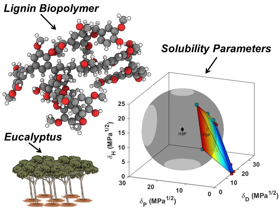
GRAPHICAL ABSTRACT
INTRODUCTION
Lignin is a plant biopolymer made from phenylpropanoid units such as guaiacyl (G), syringyl (S), and p-hydroxyphenyl (H). It is present in all terrestrial plants, including both non-wood (grasses, sugarcane, rice, and wheat) and wood (hardwoods and softwoods), and comprises roughly 10% to 30% of biomasses (Biswas et al. 2015). Industrially, lignin is obtained from a biomass pulping process, such as kraft, which is the most traditional technology. The lignin is dissolved in an aqueous solution of NaOH and Na2S (white liquor), and can then cleave β-O-4 bonds present in its native structure, generating a mixture of soluble lignin fragments (Fernández-Rodríguez et al. 2019). Then, the cellulose fibers are separated and processed for sale, while the lignin remains in a liquid phase (a weak black liquor 15% to 20% in mass) and is concentrated in a multiple effect evaporator. The heavy black liquor obtained (65% to 75% in mass) is burned to supply power to mills and to recover the cooking chemicals. Modern pulp mills, which are the most relevant in South America, produce a huge surplus of energy that is sold to the grid. The most recent mills provide power in excess of 100 MW, e.g. Puma I from Klabin SA with 150 MW of surplus (270 MW total production) (Klabin 2020). High production rates of lignin from the paper industry have encouraged the development of lignin-derived products to generate value-added materials and to provide a new source of renewable materials for the chemical industry. In 2019, approximately 20 million metric tons (T) of cellulose were produced in Brazil (Correa 2020), with 9 million T estimated for lignin, considering that this biomaterial consisted of approximately 30% hardwood (Wertz et al. 2017). For this reason, Brazil may be a strategic country for lignin production.
Applications of lignin cover many different segments because of the high concentration of phenolic groups in its structure, suggesting its use as a precursor for higher value‑added products. Some applications include its use as a dispersing agent in concrete (Mullick 1996), asphalt mixtures (Yue et al. 2019), carbon fibers (Kadla et al. 2002), polyurethanes (Gadhave et al. 2018), phenolic resins (Li et al. 2018), advanced composites (Polat et al. 2017), and antioxidants (Liu et al. 2017), among others. The remaining challenge is to provide more homogenous lignin fractions with regard to molecular size and functional groups distribution.
Many studies have performed solvent fractionation to obtain more homogeneous lignin fractions. Mörck et al. (1986) used dichloromethane (DCM), propanol, methanol, and a mixture of methanol/DCM for lignin sequential fractionation. Duval et al. (2016) used ethyl acetate, ethanol, methanol, and acetone. Ponomarenko et al. (2014) used organic solvents of increasing hydrogen-bonding ability such as: dichloromethane, n-propanol, and methanol. Cui et al. (2014) dissolved lignin in acetone and used hexane as the antisolvent to obtain the lignin fractions. Wang et al. (2018) also dissolved lignin in acetone-methanol and tetrahydrofuran-methanol, and applied hexane as the antisolvent for precipitation of the lignin fractions. However, the lack of understanding about how different solvents influence the lignin mixture partition makes it difficult to establish a rational solvent order to properly perform the sequential fractionation.
Therefore, this work aimed to contribute to the effective development of technical lignin’s fractionation by understanding how different solvents influence Eucalyptus kraft lignin partition. The solubility parameters used were Hildebrand, Hansen (HSP), and Functional (FSP).
The Hildebrand solubility parameter (or total solubility parameter) of a molecule is defined as the square root of the cohesive energy density given by the total cohesive energy (E) divided by the molar volume (V). The Hildebrand solubility parameter expands the concept of “like dissolves like” using a quantitative approach, which can be used to evaluate quantitatively the overall solubility behavior of different solutes. The Hildebrand solubility parameter can be determined experimentally for pure substances. However, when the substance degrades before vaporizing, the Hildebrand solubility parameter can be estimated using group contribution methods based on the molecular structure of the substance/solute. For lignin, the method requires determining its minimal formula (Sameni et al. 2017).
The Hansen theory is an extension of the Hildebrand theory based on the division of the total cohesive energy in three different types of molecular interactions: dispersion (δD), polar (δP), and hydrogen bonds (δH). Thus, each molecule can be represented as a point of (δD, δP, δH) coordinates in tridimensional space, or in the Hansen space.
The Hildebrand solubility parameter is related to the Hansen solubility parameter by Eq. 1. It can be interpreted as a distance between solvent points from the origin in the Hansen space. Equation 1 is as follows,
 (1)
(1)
where δ refers to Hildebrand solubility parameter, δD is the dispersive parameter, δP is the polar or dipole-dipole parameter, and δH is the hydrogen bond parameter. Usually, the solubility parameters are expressed in MPa1/2 units. E represents the total cohesive energy (J), V is the molar volume (m³/mol), ΔHvap is the molar enthalpy of vaporization, R is the ideal gas constant, and T is the absolute temperature (K).
Using the Hansen approach, a value called the interaction radius (R0) is defined, which gives the solute interaction sphere in the Hansen space. This radius is used to normalize the energy distance between the lignin HSP (δDL, δPL, δHL) and the solvents HSP (δDSi, δPSi, δHSi) in a number called relative energy difference (RED), according to Eq. 2:
 (2)
(2)
The HSP evaluation for lignin depends on the solvents that are able or not capable of dissolving it at a higher-than-arbitrary solubility threshold (ST). Then, these solvents are classified in a “good” or “bad” category, and an interaction sphere is created that includes only the “good” solvents. The center coordinates of this sphere are defined as the solute HSP (Hansen 2007; Vebber et al. 2014; Weng 2016). There is not a standard protocol to specify the ST, but it may be defined based on the degree of swelling or dissolution of solute in chosen solvents (Hansen 2007). After the sphere construction, if a solvent HSP is within the interaction sphere (RED < 1), the solvent is considered “good,” and if not, it is considered a “bad” solvent (RED > 1) for lignin dissolution.
Alternatively, the Functional solubility parameters (FSP) bypass the determination of an arbitrary solubility threshold, allowing the accurate representation of solubility data. The solubilization yield is used to create a solubility function that can be represented by a polyhedron, whose center of mass is the lignin FSP (Howell et al. 2017).
Hence, these three methodologies were applied to shed light on Eucalyptus urograndis kraft lignin solubility in organic solvents. The proper lignin solvent fractionation may allow more homogeneous lignin cuts to be obtained for use in producing lignin derivatives, which could increase the profitability of biorefineries and help establish a sustainable bio-based economy.
EXPERIMENTAL
Materials
The kraft lignin used in this work was provided by Suzano Papel e Celulose (Limeira, Brazil) from Eucalyptus urograndis black liquor. It was precipitated using a CO2 and H2SO4 solution, resulting in a composition of 94.4% lignin, 4.5% carbohydrates, and 1.1% ash.
Solubility Experiments
Solubility experiments were performed according to Duval et al. (2016) and Giummarella et al. (2016). In an Erlenmeyer flask, 5 g of lignin (mT) were mixed with 50 mL of pre-determined solvents, viz. ethyl acetate (Dinâmica Química Contemporânea LTDA, Indaiatuba SP, Brazil), acetone (Anidrol Produtos para Laboratório, Diadema SP, Brazil), butanol (Labsynth Produtos para Laboratório, Diadema SP, Brazil), cyclohexane (Anidrol Produtos para Laboratório, Diadema SP, Brazil), dichloromethane (Labsynth Produtos para Laboratório, Diadema SP, Brazil), d-limonene (Sucocítrico Cutrale, Araraquara SP, Brazil), ethanol (Êxodo Científica, Sumaré SP, Brazil), heptane (Sigma-Aldrich, St. Louis MO, USA), hexane (Dinâmica Química Contemporânea, Indaiatuba SP, Brazil), isopropanol (Labsynth Produtos para Laboratório, Diadema SP, Brazil), methanol (Anidrol Produtos para Laboratório, Diadema SP, Brazil), propanol (Labsynth Produtos para Laboratório, Diadema SP, Brazil), tetrahydrofuran (Sigma-Aldrich, St. Louis, MO, USA), and toluene (Labsynth Produtos para Laboratório, Diadema SP, Brazil). All solvents were of analytical grade. Each flask was shaken at 150 rpm for 24 h at 25 °C. The solution was filtered in a Buchner funnel using a paper filter with a pore diameter of 8 µm. The insoluble phase was left in an oven at 105 °C until reaching constant weight (mIns). Through difference of mass, the solubility yield was calculated (Eq. 3). For data evaluation, the experiments were made in duplicate and with a confidence level of 95%. Equation 3 is as follows:
Solubility Yield (%) = [ (mT – mIns) / (mT) ] × 100 (3)
Determination of Hildebrand Solubility Parameter of Kraft Lignin
For high molar mass substances, the total cohesive energy (E) can only indirectly be determined because the substances decompose before vaporizing (Gilbert 2017). That fact is true of lignin. Thus, to evaluate the kraft lignin’s Hildebrand solubility parameter, an alternative approach that considered group contribution methods can be used (Hoy 1970; Hansen 2007; Sameni et al. 2017). For this approach, a minimum chemical formula of lignin must be known in terms of its different moieties, such methoxyls and hydroxyls.
According to Gonçalves et al. (2000) and Sameni et al. (2017), the minimum formula can be determined through molar balances involving the elemental analyses of total carbon, hydrogen, nitrogen, and sulfur content (CHNS), proton nuclear magnetic resonance (1HNMR), and phosphorus nuclear magnetic resonance (31PNMR) to determine the amount of OCH3 and OH groups in lignin and heteronuclear single quantum coherence (HSQC) analyses.
CHNS analysis
The elemental analysis was performed using Vario MACRO tube (Elementar™, Langenselbold, Germany) with sulphanilamide as an internal standard. The temperature conditions were: 1150 °C for the combustion tube, 850 °C for the reduction tube, 240 °C for the CO2 tube, 150 °C for the H2O tube, and 230 °C for the SO2 tube.
The samples were conditioned in tin sheets in the shape of capsules and weighed (100 mg). The analysis was performed in duplicate, and the moisture was discounted from the hydrogen content. The oxygen content was calculated by difference.
The double bond equivalence (DBE) of lignin was calculated from carbon (C = 9) and hydrogen (H = %H/MMH) minimum quantities (Eq. 4) (Koch and Dittmar 2006):
DBE = (2C – H + 2) / 2 (4)
1HNMR and HSQC analysis
To record the 1HNMR spectrum of lignin, approximately 25 mg were dissolved in 0.60 mL of deuterated-dimethylsulfoxide (DMSO-d6). The 1HNMR spectrum was recorded on an Agilent DD2 spectrometer (Santa Clara, CA, USA), operating in Larmor frequencies of 499.726 MHz equipped with a triple resonance probe. Chemical shifts for protons were reported in ppm downfield from tetramethylsilane (TMS, 0 δ) and were referenced to the residual proton in the NMR solvent (DMSO-d6: 2.50 ppm). Carbon nuclear magnetic resonance spectra were recorded at 125.655 MHz, and chemical shifts for carbon were referenced to the carbon resonance of the solvent (DMSO-d6: 39.5 ppm). Each chemical shift range was assigned by comparison with Chen and Robert (1988).
The HSQC experiments were acquired with spectral widths of 8012.8 Hz (from 16 to 0 ppm) and 25.133 Hz (from 165 to 0 ppm) for the 1H- and 13C-dimensions, respectively. The number of collected complex points was 1202 for the 1H-dimension with a recycle delay of 1.5 s. The number of transients was 48- and 256-time increments were recorded in the 13C-dimension. The 1JC-H used was 146 Hz.
The NMR data processing used the typical matched Gaussian apodization in the 1H dimension and squared cosine-bell apodization in the 13C dimension. The data matrixes were filled with zeros up to 1202 points in the 13C-dimension, prior to the Fourier transform. The central DMSO solvent peak was used as an internal reference (δC 39.5; δH 2.50 ppm). The HSQC correlation peaks were assigned by a literature comparison (De Menezes et al. 2017). A semiquantitative analysis of the volume integrals (Wen et al. 2013) of the HSQC correlation peaks was performed using NMRPipe/NMRDraw processing software (National Institute of Standards and Technology (NIST), version 10.9, Rockville, MD, USA). The symmetric syringyl (S) and p-hydroxiphenil (H) rings contribute two C–H pairs per peak (Brandt et al. 2015), thus only the half of the full signal was used.
31PNMR analysis
This analysis was performed as done by Granata and Argyropoulos (1995) and Zawadzki and Ragauskas (2001) with modifications. In a vial, 30 mg of lignin were weighed with 100 µL of internal standard solution endo-hydroxy-5-norbornene-2,3-dicarboxylic acid imide (135 mM in dimethylformamide), 400 µL of a mixture of deutered piridine and chloroform (1.6:1 v/v stored under molecular sieves), and 100 µL of relaxation agent chromium(III) acetylacetonate (16.35 mM in deutered piridine/chloroform, 1.6:1v/v). After lignin dissolution, 100 µL of phosphitylation agent 2-chloro-4,4,5,5-tetramethyl-1,3,2-dioxaphospholane was added, and the solution was transferred to a 5-mm NMR tube. The analysis was conducted by a Bruker Avance III – 9.4 Tesla spectrometer (Billerica, MA, USA; 400.13 MHz for 1-H frequency), with a probe PABBI (5 mm) and automatic tuning and matching (ATMA). The pulse sequence was zgpg30.
A total of 512 scans (ns) were made with 64 k points (td) in a spectral width (sw) of 350 ppm and receptor gain (rg) of 1820. The time between each acquisition (d1) was 25 s, and the time of acquisition (aq) was approximately 0.57 s. The total time of acquisition was 3 h and 38 min. The processing of spectra was made with 32k (SI), using an exponential multiplication with lb = 1.0 Hz, the phase and baseline automatically adjusted.
The semiquantitative analysis was made by integrating the respective regions of chemical groups (Granata and Argyropoulos 1995). The Hildebrand parameter was calculated using a group attribution chart presented by Sameni et al. (2017) (Eq. 5),
 (5)
(5)
where δ is the Hildebrand solubility parameter, N is the quantity of each group in minimum formula according to Sameni et al. (2017), and Δe and ΔV are respectively the cohesive energy and molar volume contribution of each group.
Determination of Hansen Solubility Parameters (HSP) of Kraft Lignin
Hansen solubility parameters of kraft lignin were calculated from experimental solubility data, using the algorithm proposed by Gharagheizi (2007) written in Matlab (MathWorks, version 2019a, Natick, MA, USA). The Nelder-Mead method was used for the global minimal search of the objective function. The solubility parameters of the solvents (δDS, δPS, δHS) were obtained from Hansen (2007), and the first guess for the lignin HSP calculation was the mean of each solvent HSP. As the solubility threshold is an arbitrary factor, a set of values were explored (0%, 25%, 30%, 50%, 75%, and 100%) to understand its influence on the lignin HSP determination. If the lignin solubility yield was higher than the threshold in a given solvent, its solubility (s) was considered 1, otherwise it was considered 0. This procedure was performed for all solvents used in this work (n = 14).
Determination of Functional Solubility Parameters (FSP) of Kraft Lignin
The FSP were calculated using the solvents HSP and lignin solubility yields in each solvent. The code implemented was proposed by Howell et al. (2017), and the lignin solubility region was represented by a polyhedron using a Delaunay triangulation in the Matlab environment. The software FreeFEM++ (FreeFEM, version 4.6, Paris, Île-de-France, France) was used to calculate the FSP of lignin and its gradient solubility in tridimensional space using numerical integration.
The cross-sections in this polyhedron were made using a function to determine the intersection contour between the object and a plane (Pariterre 2020). Then, the solubility yield was calculated by the linear interpolation of the lignin solubility in the contour.
RESULTS AND DISCUSSION
Kraft Lignin Experimental Solubility Yields in Organic Solvents
Kraft lignin solubility yields varied from 3.4% to 95.4% (Table 1). As expected, the use of hydrocarbons to dissolve lignin presented low yields (3.4% to 9.4%) due to the low affinity between the phenylpropanoid units and nonpolar solvents. For alcoholic solvents, the lignin solubility yield decreased with the increase of carbon chain length, which can be attributed to hydrogen and/or polar intermolecular forces that were inversely proportional to the aliphatic hydrocarbon side chain size (Duval et al. 2016).
Table 1. Eucalyptus urograndis Kraft Lignin Experimental Solubility Yield in Organic Solvents

*Hansen solubility parameters of solvents (Hansen 2007)
The molecular geometry was another factor that influenced the interaction of lignin with organic solvents. For example, isopropanol had lower solubility yield than its isomer n-propanol. These substances presented different molar volumes and solubility parameters (isopropanol V = 76.8 cm³/mol, δ = 22.7 MPa½, and n-propanol V = 75.2 cm³/mol, δ = 24.6 MPa½) (Hansen 2007), as the magnitude of the intermolecular forces decreases with the branching degree of the substance. Then, the number of isopropanol molecules that reached the lignin structure core decreased in comparison with the linear molecule of n-propanol. Additionally, this may have indicated that isopropanol entered the lignin structure in a particular orientation where the entropy factor contributed to the reduced solubility (Laprade et al. 1977).
The solubility yields of this lignin were compared with Duval et al. (2016) (Fig. 1). The trend in both works was similar, whereby tetrahydrofuran, methanol, and acetone presented the highest solubility yields. The solubility yield in ethyl acetate, isopropanol, and n-propanol were similar even given the difference in wood species; this work studied hardwood lignin, and Duval et al. (2016) studied softwood lignin. The higher solubility of Eucalyptus kraft lignin, in comparison with the respective study done with softwood kraft lignin, may be attributed to the smaller average molecular mass of Eucalyptus kraft lignin of Mw = 2138 Da, while softwood was Mw = 6500 Da.

Fig. 1. Comparison of the solubility yield of lignins in different solvents; () Eucalyptus urograndis (hardwood; the present study), () softwood (Duval et al. 2016)
The lignin solubility yield was plotted versus each solvent HSP (Fig. 2) and a multiregression analysis was performed (Table 2) to investigate whether these parameters could explain the solubility yield in a linear mathematical model (Eq. 6),
Solubility Yield (%) = ( ![]() δD +
δD + ![]() δP +
δP + ![]() δH + ε) × 100 (6)
δH + ε) × 100 (6)
where δD refers to the dispersion parameter; δP refers to the polar parameter; δH refers to the hydrogen bond parameter of solvents; and , , refer to adjustable parameters of the mathematical model. The error is represented by ε.

Fig. 2. The correlation of the solubility yield of lignin with the solvents HSP: a) δD, b) δP, c) δH, and d) δ; the shaded region represents the 95% confidence interval
Table 2. Analysis of Variance of the Solubility Yield

Note: df: degrees of freedom; SS: sum of squares: MS: mean squares; Multiple R = 0.852; R² = 0.725; Adjusted R² = 0.643; Standard error = 0.207; Observations = 14
In the multilinear regression, the polar parameter of solvents (δP) was the only one that had statistical evidence to explain the solubility yield of lignin in organic solvents according to analysis of variance (ANOVA) statistics (p-value < 0.05). However, lignin is a biomaterial with high quantities of aliphatic and phenolic hydroxyl groups, and therefore the hydrogen bond between lignin and polar solvents occurs. For this reason, it was expected that δH would be a contributing factor in the solubility (Duval et al. 2016). However, its statistics revealed weak association between these variables. This may explain the similar solubility yields of kraft lignin in aprotic solvents (tetrahydrofuran and acetone) and protic solvents (ethanol and methanol), all of which had different capabilities of forming hydrogen bonds.
To refine the lignin solubility yield prediction, a second model was proposed that removed the variables without influence on the results (Eq. 7). In that model, only the polar parameter was considered (Table 3):
Solubility Yield (%) = ( βδP + ε) × 100% (7)
Table 3. Analysis of Variance of the Solubility Yield with Only the δP Contribution

Note: df: degrees of freedom; SS: sum of squares: MS: mean squares; Multiple R = 0.826; R² = 0.682; Adjusted R² = 0.655; Standard error = 0.203; Observations = 14
The significance F and β p-value of this second correlation were nearly 10 times lower than the first, revealing an improvement in the statistical model relevance.
Hildebrand Solubility Parameter of Kraft Lignin
The group contribution method was used to calculate the Hildebrand parameter of kraft lignin (δ). The first step was reducing all structural complexity of lignin polyphenolic mixture into a single minimum formula.
CHNS results
The kraft lignin of this work presented 64.8% carbon, 6.0% hydrogen, 0.2% nitrogen, and 2.2% sulfur, determined by CHNS elemental analysis, and 26.8% oxygen, determined by difference. In general, biomasses have high carbon content, a characteristic that was observed in this material. The sulfur content originated from the hydrosulfide group (HS–), specifically, from the cooking liquor present in kraft pulping, and was covalently bonded to lignin structure. There was minimum nitrogen content, which was associated to proteins that were present in the original biomass. The oxygen content represented all oxygenated groups in the lignin structure, such as aliphatic and aromatic hydroxyls, ethers, methoxyls, and carboxylic units.
The DBE was determined for the contribution of C= groups in the Hildebrand solubility parameter calculation. The DBE directly correlates to both the aromaticity and degree of condensation of lignins (Kim et al. 2014). In this work, the DBE was 5.03, which agreed with the results found in Sameni et al. (2017) that determined hardwood kraft lignin DBE as 5.35.
¹HNMR results
The kraft lignin was characterized by the 1HNMR spectrum (Fig. 3) with regions corresponding to nonoxygenated aliphatic, methoxyl, aliphatic, aromatic, carboxylic, and aldehyde groups. The spectrum was normalized to the most intense peak. Water and DMSO peaks were excluded from calculation of specific groups, and the semiquantitative analysis was performed (Table 4).

Fig. 3. The 1HNMR spectrum of Eucalyptus urograndis kraft lignin
Table 4. Lignin Group Content Obtained from the 1HNMR Spectrum

*Chen and Robert (1988)
With the semi-quantification of the methoxyl region, and the carbon, hydrogen, and oxygen contents by CHNS analysis, a general chemical formula of the lignin was achieved through molar balances: C9H7.1O1.8(OCH3)1.5. This formula was similar to that of other hardwood lignin (Table 5).
Table 5. Minimum Formula Comparison of Lignins from Different Sources

HSQC results
The HSQC spectrum of lignin was divided into aliphatic and aromatic parts (Figs. 4 and 5) and some structures were identified, including methoxyls, and Cβ-Hβ in β-O-4 and in resinol structures (71.8/4.85 and 84.8/4.65 ppm, respectively). Some C2−H2, C3−H3, and C4−H4 bonds were found in 72.9/3.14, 74.1/3.32, and 75.6/3.63 ppm, respectively, associated to polysaccharide fragments, such as β-D-xylopyranoside, attached in lignin (De Menezes et al. 2017).

Fig. 4. The HSQC of the Eucalyptus urograndis kraft lignin (aliphatic)

Fig. 5. The HSQC of the Eucalyptus urograndis kraft lignin (aromatic)
The syringyl (S) and guayacil (G) units were characterized and semi-quantified in the aromatic region of the HSQC spectrum. These units had different molar volumes, and it was necessary to determine their proportion to incorporate in the Hildebrand parameter calculation. The content of S and G units were 68.3% and 31.7%, respectively, with the S/G ratio of 2.15, which agreed with literature (Anderson et al. 2019) and reflects the source of lignin (hardwood) (Faix 1991). The p-hydroxyphenyl unit (H) may have had a small presence in the lignin composition because it was not found in the spectra.
31PNMR results
The oxygen content presented in CHNS analysis reflected the total oxygen content in lignin. However, each hydroxyl group (aliphatic, phenolic, and carboxylic) had different contributions in the Hildebrand parameter calculation. Thus, the 31PNMR spectrum (Fig. 6) was obtained for lignin and the quantity of each hydroxyl groups was determined (Table 6).
Table 6. Hydroxyl Content of Kraft Lignin Obtained from the 31PRMN Spectrum

*According to Granata and Argyropoulos (1995)

Fig. 6. 31PRMN spectrum of Eucalyptus urograndis kraft lignin
The p-hydroxyphenyl OH (H unit) corresponded to 2.8% of the total phenolic hydroxyl content. This may explain the HSQC results, as p-hydroxyphenyl OH can be present in minimal quantities.
Extended minimum formula and Hildebrand parameter
The extended minimum formula of kraft lignin was determined with the inclusion of some lignin moieties such the aliphatic, aromatic, and carboxylic OH (Eq. 8).
 (8)
(8)
The Hildebrand solubility parameter of Eucalyptus urograndis Kraft lignin was 27.3 MPa1/2 (Table 7). This value is comparable to other works that presented values between 24 and 31 MPa1/2 for kraft lignins (Ni and Hu 1995; Thielemans and Wool 2005; Quesada-Medina et al. 2010; Wang et al. 2011; Sameni et al. 2017).
The Hildebrand solubility parameter value explained the high lignin solubility yields in methanol (δ = 29.6 MPa1/2) and ethanol (δ = 26.5 MPa1/2), as both have solubility parameters closer to the parameter obtained. However, the Hildebrand solubility parameter fails to describe the solubility behavior of lignin in acetone (δ = 19.9 MPa1/2) and tetrahydrofuran (δ = 19.5 MPa1/2) that presented high lignin solubility yields, 88.8% and 75.4%, respectively.
As the δ parameter was unable to describe lignin solubility in all these solvents, the Hansen method was used to deepen this investigation.
Table 7. Cohesive Energy (Δe) and Molar Volume (ΔV) in Lignin Groups

*According to Sameni et al. (2017); N is the quantity of each group in minimum formula
Hansen Solubility Parameter of Kraft lignin
The “good” or “bad” solvents’ classification in each solubility threshold (ST) is presented in Table 8, while lignin’s HSP (δDL, δPL, δHL) and R0 determination in each ST are presented in Table 9. Considering the entire solubility threshold range, δD of the lignin was similar (from 13.5 to 22.1 MPa1/2), whereas the other parameters vary considerably (5.0 < δP < 40.5 and 6.2 < δH < 12.1 MPa1/2). The lignin HSP varied with the solubility threshold because of different conditions that must be satisfied to place the “good” solvents’ points inside the sphere, whereas the other solvents must be outside.
For this reason, different HSPs were obtained depending on the coordinates of the sphere created. As discussed in Hansen (2007), the HSP parameters usually vary between correlations based on the same data when different solubility thresholds are used. This variability was observed in the lignin studied in the present study, and may explain the variation observed in the HSP. In this complex material, some polyphenolic molecules may be extracted in some solvents rather than others.
Table 8. Classification of the Solvents (“Good” = 1 and “Bad” = 0) Using Different ST

Table 9. HSP for Kraft Lignin Using Different ST

In addition, previous studies have calculated lignin’s HSP from different sources (Table 10). Lignin is a macromolecule consisting of various non-regular structures (monolignols and interunit linkages), and this composition can also explain the variation of the solubility parameters depending on the lignin source. The results from previous studies differ because lignins may present distinct characteristics depending on their source, and thus reflect variations in the H, G, and S unit compositions and molecular sizes.
Table 10. HSP of Lignins from Different Sources

*Considering 70% of the delignification extent minimum as the solubility threshold
In Novo and Curvelo’s research (2019), the HSPs of organosolv sugarcane lignin were calculated based on the minimum delignification extent as the solubility threshold. Hansen (2007) determined the HSP for milled wood lignin (δD = 21.9, δP = 14.1, δH = 16.9, and R0 = 13.7 MPa½), but the solubility threshold was not clearly stated. Other works, such as Vebber et al. (2014) and Weng (2016), also determined the HSP using the same data and presented similar values with modified algorithms. In this work, the values of δ and R0 were closer to these works considering ST = 30%.
The δP and R0 values of Eucalyptus urograndis kraft lignin in this study were higher than those for sugarcane bagasse lignin in Novo and Curvelo’s work (2019), considering the same ST. However, the δH was the opposite because the content of monolignols varies between species. Eucalyptus has an abundance of S and G units, whereas sugarcane bagasse has a predominance of H units. This difference may explain the difference in HSP, even if the δH of H units was slightly higher than S and G units (Hansen 2007).
The Hansen sphere for kraft lignin when ST = 30% is presented in Fig. 7 to illustrate the solvent position inside and outside the sphere.

Fig. 7. The Hansen sphere for kraft lignin with a solubility threshold of 30% ( is outside the sphere and is inside the sphere); a) δDδPδH ; b) δH vs. δD ; c) δH vs. δP ; d) δD vs. δP
In addition, the RED was calculated for each solubility threshold (Table 11). The higher the solubility threshold, the greater the RED. For ST = 0%, all solvents were considered “good,” justifying RED < 1. For ST = 100%, all solvents were considered “bad” because none of them were able to solubilize kraft lignin completely, resulting in RED > 1.
For intermediate values of the solubility threshold (25% < ST < 75%), some solvents were considered “good” and some “bad,” but tetrahydrofuran, methanol, ethanol, and acetone presented RED ≤ 1 in this whole interval, demonstrating they are “good” solvents for the dissolution of kraft lignin, even with distinct δH/δP values.
Although high-solubility solvents were inside the interaction sphere (THF, methanol, acetone, and ethanol), the RED results revealed that the definition of the solubility threshold is crucial to define “good” and “bad” solvents. For example, the dissolution of lignin in ethyl acetate was considered “good” at ST = 25% and “bad” at ST = 30%. For this reason, to overcome the limitations caused by an arbitrary solubility threshold, another method had to be used.
Table 11. RED of Solvents Varying the ST at 25 °C

FSP of Kraft lignin
The lignin solubility region determined by the FSP approach is presented in Fig. 8 where this polyhedron is the “shell” of the solubility function.

Fig. 8. Polyhedron constructed for FSP evaluation of kraft lignin including all solvents: a) δDδPδH, b) δH vs. δD, c) δH vs. δP, and d) δD vs. δP
In this representation, the highest solubility yield of lignin was found in the vertices farthest from δD axis that were from ethanol and methanol HSP. However, the lignin solubility yield in acetone and tetrahydrofuran (THF) was not found because its HSP points were located inside the polyhedron. In that case, the highest solubility appeared to be in the alcohols.
This “shell” obstructed the full analysis of the lignin solubility function because it suppressed the internal gradients of this polyhedron. In that instance, perpendicular cross sections were cut to provide greater detail, thus enhancing the analysis (Fig. 9).

Fig. 9. Polyhedron cross-sections along: a) δD axis, b) δP axis, and c) δH axis
In Fig. 9a, the solubility yield gradients in the cross-sections were similar to Fig. 8c, where the gradient behavior did not change along the δD axis. Instead, the main variations of the solubility yields were in the δP and δH directions.
In Fig. 9b, with the gradient along the δH and δD axes, some tendencies were observed solely near to the highest solvent δP, where the solubility increased along the δH axis. In addition, some high solubility of lignin was found in the cross-section of δP ≈ 3.2 MPa½, which was closer to the THF δP = 5.7 MPa½. The solubility function indicated that the lignin may have had at least two independent high solubility regions and, for this reason, its interaction was higher with protic solvents (alcohols) and aprotic solvents (THF and acetone) that have HSP close to those solubility regions.
In Fig. 9c, with the cross-section gradients along the δP and δD axis, it was confirmed that the solubility yield gradient increased towards in δP direction regardless of δH. For this reason, the solubility yield of this lignin was more proportional to solvents δP than δH, corroborating with the previous results given by multiregression analyses.
The lignin FSP were δD = 16.0 MPa1/2, δP = 7.1 MPa1/2, and δH = 10.4 MPa1/2, defined as the center of mass of the polyhedron because it is the “central tendency” of the function’s behavior according to Howell et al. (2017). The Hildebrand parameter obtained through this method was δ = 20.4 MPa1/2, explaining the high solubility yield of lignin in THF (95.4%, δ = 19.5 MPa1/2) and acetone (88.4%, δ = 19.9 MPa1/2) due to the proximity between the solvents and lignin Hildebrand parameters.
However, comparing the Hildebrand parameters of the solvents and the FSP the solubility yields of lignin in alcohols was not justified by this method. The group contribution, HSP, and FSP methods all failed to agree with the prediction of the solubility of lignin in all solvents studied.
Comparison between Methods
The calculated lignin solubility parameters were distinct among the three methods (Table 12). The Hildebrand parameter ranged from 19.1 to 43.1 MPa1/2 and the R0 from 6.9 to 35.4 MPa1/2 because of the solubility threshold considered.
Table 12. Comparison of the Solubility Parameters of Lignin Determined by Different Methodologies

The Hildebrand parameter calculated from the group contribution did not have geometrical representation. The Hansen and Functional methods presented a tridimensional perspective of the solubility of lignin in the organic solvents studied.
The Hansen approach defined a unique solubility region for lignin, and the calculated HSP varied because of the definition of “good” solvents. In contrast, the Functional approach determined that lignin may have at least two high solubility yield regions, and thus the center of mass was found between those regions.
Accordingly, the variation in parameters may have influenced the choice of solvents to perform lignin fractionation. However, the polyhedron constructed was a more reliable method to predict the solubility in organic solvents. Therefore, it was concluded that defining unique solubility parameters for lignin (δDL, δPL, δHL) may not be an ideal tool to predict lignin solubility in all organic solvents.
Although it was not possible to find solubility parameters that perfectly determined the solubility of lignin in certain solvents, the review of each method showed that some methods were better than others for this purpose.
CONCLUSIONS
- The lignin in this study presented high experimental solubility yields in alcohols, THF, and acetone that were visualized as two high solubility regions in polyhedron built using the FSP approach. The Hildebrand parameter explained the high experimental solubility yields of kraft lignin in methanol and ethanol, while the FSP explained the high experimental solubility yields in THF and acetone.
- The variation obtained in the lignin HSP method suggested that its calculation and comparison must be done admitting the same solubility threshold.
- Solvents δP were in agreement with the solubility yield results of polar protic and aprotic solvents.
- The polyhedron used for the FSP better represented the solubility region of lignin compared to the Hildebrand and Hansen theories. It can be used to predict lignin solubility in organic solvents and to evaluate the best solvents for lignin fractionation.
ACKNOWLEDGMENTS
The authors are grateful for the support of the Conselho Nacional de Desenvolvimento Científico e Tecnológico (CNPq) for financial support (Process number: 133196/2018-6), the Coordenação de Aperfeiçoamento de Pessoal de Nível Superior (CAPES) for financial support (PROEX 0886/2018), Suzano Papel e Celulose for 31PNMR analysis, and the Brazilian Biosciences National Laboratory (Brazilian Center for Research in Energy and Materials – CNPEM) for HSQC and 1HNMR analyses.
REFERENCES CITED
Anderson, E. M., Stone, M. L., Katahira, R., Reed, M., Muchero, W., Ramirez, K. J., Beckham, G. T., and Román-Leshkov, Y. (2019). “Differences in S/G ratio in natural poplar variants do not predict catalytic depolymerization monomer yields,” Nature Communications 10(1), Article No. 2033. DOI: 10.1038/s41467-019-09986-1
Biswas, R., Uellendahl, H., and Ahring, B. K. (2015). “Wet explosion: A universal and efficient pretreatment process for lignocellulosic biorefineries,” BioEnergy Research 8(3), 1101-1116. DOI: 10.1007/s12155-015-9590-5f
Brandt, A., Chen, L., Van Dongen, B. E., Weltoon, T., and Hallett, J. P. (2015). “Structural changes in lignins isolated using an acidic ionic liquid water mixture,” Green Chemistry 17(11), 5019-5034. DOI: 10.1039/c5gc01314c
Chen, C. L., and Robert, D. (1988). “Characterization of lignin by 1H and 13C NMR spectroscopy,” Methods in Enzymology 161, 137-174. DOI: 10.1016/0076-6879(88)61017-2
Correa, C. (2020). Cenários Ibá: Statistics of the Brazilian Tree Industry – 1st Quarter 2020, Brazilian Tree Industry (Ibá), Brasília, DF, Brazil.
Cui, C., Sun, R., and Argyropoulos, D. S. (2014). “Fractional precipitation of softwood kraft lignin: Isolation of narrow fractions common to a variety of lignins,” ACS Sustainable Chemistry & Engineering 2(4), 959-968. DOI: 10.1021/sc400545d
De Menezes, F. F., Rencoret, J., Nakanishi, S. C., Nascimento, V. M., Silva, V. F. N., Gutiérrez, A., Del Río, J. C., and De Moraes Rocha, G. J. (2017). “Alkaline pretreatment severity leads to different lignin applications in sugar cane biorefineries,” ACS Sustainable Chemistry & Engineering 5(7), 5702-5712. DOI: 10.1021/acssuschemeng.7b00265
Duval, A., Vilaplana, F., Crestini, C., and Lawoko, M. (2016). “Solvent screening for the fractionation of industrial kraft lignin,” Holzforschung 70(1), 11-20. DOI: 10.1515/hf-2014-0346
Faix, O. (1991). “Classification of lignins from different botanical origins by FT-IR spectroscopy,” Holzforschung 45(1), 21-27. DOI: 10.1515/hfsg.1991.45.s1.21
Fernández-Rodríguez, J., Erdocia, X., Hernández-Ramos, F., Alriols, M. G., and Labidi, J. (2019). “Lignin separation and fractionation by ultrafiltration,” in: Separation of Functional Molecules in Food by Membrane Technology, C. M. Galanakis (ed.), Academic Press, Cambridge, MA, USA, pp. 229-265. DOI: 10.1016/B978-0-12-815056-6.00007-3
Gadhave, R. V., Mahanwar, P. A., and Gadekar, P. T. (2018). “Lignin-polyurethane based biodegradable foam,” Open Journal of Polymer Chemistry 8(1), 1-10. DOI: 10.4236/ojpchem.2018.81001
Gharagheizi, F. (2007). “New procedure to calculate the Hansen solubility parameters of polymers,” Journal of Applied Polymer Science 103(1), 31-36. DOI: 10.1002/app.23874
Gilbert, M. (2017). “Relation of structure to chemical properties,” in: Brydson’s Plastics Materials, Butterworth-Heinemann, Oxford, UK, pp. 75-102. DOI: 10.1016/B978-0-323-35824-8.00005-0
Giummarella, N., Lindgren, C., Lindström, M. E., and Henriksson, G. (2016). “Lignin prepared by ultrafiltration of black liquor: Investigation of solubility, viscosity, and ash content,” BioResources 11(2), 3494-3510. DOI: 10.15376/biores.11.2.3494-3510
Gonçalves, A. R., Schuchardt, U., Bianchi, M. L., and Curvelo, A. A. S. (2000). “Piassava fibers (Attalea funifera): NMR spectroscopy of their lignin,” Journal of the Brazilian Chemical Society 11(5), 491-494. DOI: 10.1590/S0103-50532000000500010
Granata, A., and Argyropoulos, D. S. (1995). “2-Chloro-4,4,5,5-tetramethyl-1,3,2-dioxaphospholane, a reagent for the accurate determination of the uncondensed and condensed phenolic moieties in lignins,” Journal of Agricultural and Food Chemistry 43(6), 1538-1544. DOI: 10.1021/jf00054a023
Hansen, C. M. (2007). “Hansen solubility parameters—Biological materials,” in: Hansen Solubility Parameters: A User’s Handbook, CRC Press, Boca Raton, FL, USA, pp. 269-292. DOI: 10.1201/9781420006834
Howell, J., Roesing, M., and Boucher, D. S. (2017). “A functional approach to solubility parameter computations,” The Journal of Physical Chemistry 121(16), 4191-4201. DOI: 10.1021/acs.jpcb.7b01537
Hoy, K. L. (1970). “New values of the solubility parameters from vapor pressure data,” Journal of Paint Technology 42(541), 76-118.
Kadla, J. F., Kubo, S., Venditti, R. A., Gilbert, R. D., Compere, A. L., and Griffith, W. (2002). “Lignin-based carbon fibers for composite fiber applications,” Carbon 40(15), 2913-2920. DOI: 10.1016/S0008-6223(02)00248-8
Kim, J. Y., Hwang, H., Oh, S., Kim, Y. S., Kim, U. J., and Choi, J. W. (2014). “Investigation of structural modification and thermal characteristics of lignin after heat treatment,” International Journal of Biological Macromolecules 66, 57-65. DOI: 10.1016/j.ijbiomac.2014.02.013
Klabin (2020). “About Puma I,” Klabin SA, (https://projetopuma.klabin.com.br/sobre-o-puma-i), Accessed 22 September 2020.
Koch, B. P., and Dittmar, T. (2006). “From mass to structure: An aromaticity index for high-resolution mass data of natural organic matter,” Rapid Communication in Mass Spectrometry 20(5), 926-932. DOI: 10.1002/rcm.2386
Laprade, B., Mauger, T. W., Petersen, H., Lausier, J. M., and Paruta, A. N. (1977). “Solubility for normal and branched chain alkyl barbiturates in water. II. Relationship with apparent molar volume,” Drug Development and Industrial Pharmacy 3(1), 73-85. DOI: 10.3109/03639047709055606
Li, R. J., Gutierrez, J., Chung, Y., Frank, C. W., Billington, S. L., and Sattely, E. S. (2018). “A lignin-epoxy resin derived from biomass as an alternative to formaldehyde-based wood adhesives,” Green Chemistry 20(7), 1459-1466. DOI: 10.1039/C7GC03026F
Liu, D., Li, Y., Qian, Y., Xiao, Y., Du, S., and Qiu, X. (2017). “Synergistic antioxidant performance of lignin and quercetin mixtures,” ACS Sustainable Chemistry & Engineering 5(9), 8424-8428. DOI: 10.1021/acssuschemeng.7b02282
Morais, S. A. L. (1992). Contribuição ao Estudo Químico e Espectroscópico da Lignina de Madeira Moída do Eucalyptus grandis: Isolamento, Quantificação e Análise Estrutural [Contribution to the Chemical and Spectroscopic Study of Eucalyptus grandis Milled Wood Lignin: Isolation, Quantification and Structural Analysis], Ph.D. Dissertation, Universidade Federal de Minas Gerais, Belo Horizonte, MG, Brazil.
Morais, S. A., Nascimento, E. A., and Melo, D. C. (2005). “Análise da madeira do Pinus oocarpa, Parte II – Caracterização estrutural da lignina de madeira moída [Chemical naalysis of the Pinus oocarpa wood, Part II – Characterization of the milled wood lignin],” Revista Árvore 29(3), 471-478. DOI: 10.1590/S0100-67622005000300015
Mörck, R., Yoshida, H., Kringstad, K. P., and Hatakeyama, H. (1986). “Fractionation of kraft lignin by successive extraction with organic solvents. I. Functional groups, 13C-NMR-spectra and molecular weight distributions,” Holzforschung 40(Suppl.), 51-60.
Mullick, A. K. (1996). “Use of lignin-based products in concrete,” in: Waste Materials Used in Concrete Manufacturing, S. Chandra (ed.), William Andrew Publishing, Norwich, NY, USA, pp. 352-429. DOI: 10.1016/B978-081551393-3.50010-7
Ni, Y., and Hu, Q. (1995). “Alcell® lignin solubility in ethanol–water mixtures,” Journal of Applied Polymer Science 57(12), 1441-1446. DOI: 10.1002/app.1995.070571203
Novo, L. P., and Curvelo, A. A. S. (2019). “Hansen solubility parameters: A tool for solvent selection for organosolv delignification,” Industrial & Engineering Chemistry Research 58(31), 14520-14527. DOI: 10.1021/acs.iecr.9b00875
Pariterre (2020). “sliceDelaunay,” MathWorks, (https://www.mathworks.com/matlabcentral/fileexchange/56536-slicedelaunay), Accessed 04 July 2020.
Polat, Y., Stojanovska, E., Negawo, T. A., Doner, E., and Kilic, A. (2017). “Lignin as an additive for advanced composites,” in: Green Biocomposites: Manufacturing and Properties, M. Jawaid, S. M. Sapuan, and O. Y. Alothman (eds.), Springer, Cham, New York, NY, USA. DOI: 10.1007/978-3-319-46610-1_4
Ponomarenko, J., Dizhbite, T., Lauberts, M., Viksna, A., Dobele, G., Bikovens, O., and Telysheva, G. (2014). “Characterization of softwood and hardwood LignoBoost kraft lignins with emphasis on their antioxidant activity,” BioResources 9(2), 2051-2068. DOI: 10.15376/biores.9.2.2051-2068
Quesada-Medina, J., López-Cremades, F. J., and Olivares-Carrillo, P. (2010). “Organosolv extraction of lignin from hydrolyzed almond shells and application of the δ-value theory,” Bioresource Technology 101(21), 8252-8260. DOI: 10.1016/j.biortech.2010.06.011
Sameni, J., Krigstin, S., and Sain, M. (2017). “Solubility of lignin and acetylated lignin in organic solvents,” BioResources 12(1), 1548-1565. DOI: 10.15376/biores.12.1.1548-1565
Thielemans, W., and Wool, R. P. (2005). “Lignin esters for use in unsaturated thermosets: Lignin modification and solubility modeling,” Biomacromolecules 6(4), 1895-1905. DOI: 10.1021/bm0500345
Vebber, G. C., Pranke, P., and Pereira, C. N. (2014). “Calculating Hansen solubility parameters of polymers with genetic algorithms,” Journal of Applied Polymer Science 131(1), Article ID 39696. DOI: 10.1002/app.39696
Wang, Q., Chen, K., Li, J., Yang, G., Liu, S., and Xu, J. (2011). “The solubility of lignin from bagasse in a 1,4-butanediol/water system,” BioResources 6(3), 3034-3043. DOI: 10.15376/biores.6.3.3034-3043
Wang, Y. Y., Li, M., Wyman, C. E., Cai, C. M., and Ragauskas, A. J. (2018). “Fast fractionation of technical lignin by organic cosolvents,” ACS Sustainable Chemistry & Engineering 6(5), 6064-6072. DOI: 10.1021/acssuschemeng.7b04546
Wen, J. L., Sun, S. L., Xue, B. L., and Sun, R. C. (2013). “Recent advances in characterization of lignin polymer by solution-state nuclear magnetic resonance,” Materials 6(1), 359-391. DOI: 10.3390/ma6010359
Weng, M. (2016). “Determination of the Hansen solubility parameters with a novel optimization method,” Journal of Applied Polymer Science 133(16), Article ID 43328. DOI: 10.1002/app.43328
Wertz, J., Deleu, M., Coppée, S., and Richel, A. (2017). “Valorization of lignin,” in: Hemicelluloses and Lignin in Biorefineries, CRC Press, Boca Raton, FL, USA, pp. 245-265. DOI: 10.1201/b22136
Yue, Y., Abdelsalam, M., Luo, D., Khater, A., Musanyufu, J., and Chen, T. (2019). “Evaluation of the properties of asphalt mixes modified with diatomite and lignin fiber: A review,” Materials 12(3), Article number 400. DOI: 10.3390/ma12030400
Zawadzki, M., and Ragauskas, A. (2001). “N-Hydroxy compounds as new internal standards for the ³¹P-NMR determination of lignin hydroxyl functional groups,” Holzforschung 55(3), 283-285. DOI: 10.1515/HF.2001.047
Article submitted: June 6, 2020; Peer review completed: August 15, 2020; Revised version received and accepted: August 23, 2020; Published: September 23, 2020.
DOI: 10.15376/biores.15.4.8577-8600