Space-time analysis of the longitudinal variation in wood specific gravity of teak and its effect on tree growth and development

Adutwum, J. O., Sakagami, H., Koga, S., and Matsumura, J. (2023). “Space-time analysis of the longitudinal variation in wood specific gravity of teak and its effect on tree growth and development,” BioResources 18(2), 2670-2692.

Abstract

The space-time structure of a teak wood specific gravity (SG) dataset was analyzed using a mixed-effects model. Spatial correlation increased in space, a phenomenon attributable to the maturation of apical meristems, while the temporal correlation of vascular meristems decreased over time. The decay of temporal correlation over time was attributed to the diminishing crown effect on the later formed wood further away from the pith, morphogen gradient, and probably changing microenvironmental conditions. The Kronecker product was used to collect spatiotemporal data on the intricate dynamic process of the evolution of the apical and lateral meristems. The results showed that height and relative radial distance (RRD) (i.e., the flow of time with wood formation) were statistically significant factors, with their interaction showing no significance. The results confirm the usefulness of using the space-time approach to elucidate the interaction between the apical and lateral meristems, two major inherent biological systems that control tree growth and wood formation dynamics. To understand the origins of patterns that vary both temporally and spatially in the tree, future work should describe the variation of SG within the tree due to increasing height (space) and diameter (age) as a matrix; then the correlation function can be modelled.

Download PDF

Full Article

Space-time Analysis of the Longitudinal Variation in Wood Specific Gravity of Teak and Its Effect on Tree Growth and Development

Jerry Oppong Adutwum,^a Hiroki Sakagami,^b Shinya Koga,^c and Junji Matsumura ^d,*

DOI: 10.15376/biores.18.2.2670-2692

Keywords: Juvenility; Kronecker product; Maturation; Mixed-effects model; Space-time dynamics; Stochastic processes; Teak; Tree growth; Wood specific gravity

Contact information: a: Graduate School of Bioresource and Bioenvironmental Sciences, Faculty of Agriculture, Kyushu University, 744 Motooka, Nishi-ku, Fukuoka 819-0395; b: Laboratory of Wood Materials Technology, Faculty of Agriculture, Kyushu University, 744 Motooka, Nishi-ku, Fukuoka 819-0395; c: Laboratory of Forest Resources Management, Faculty of Agriculture, Kyushu University, Fukuoka 811-2415; d: Laboratory of Wood Science, Faculty of Agriculture, Kyushu University, 744 Motooka, Nishi-ku, Fukuoka 819-0395; *Corresponding author: matumura@agr.kyushu-u.ac.jp

GRAPHICAL ABSTRACT

INTRODUCTION

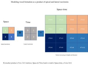
Teak (Tectona grandis L.f) is a highly valued tropical timber species that is widely grown in regions within its native habitat in Southeast Asia, specifically India, Laos, Myanmar, and Thailand, as well as in Latin America, Africa, and Oceania (Gaitan-Alvarez et al. 2019; Moya and Tenorio 2021; Sasidharan 2021). There has been a significant amount of research on the radial properties of teak wood, while the longitudinal variations have received relatively little attention, as recently summarized by Moya and Tenorio (2021). In the context of the above information, the growth pattens of teak in both spatial (height) and temporal (diameter/radial) dimensions are characterized jointly, i.e., the organization of growth pattens in both space and time into a hierarchical system, using tensor and vector calculus principles. This approach involves understanding the complex dynamics of tree growth and development processes and using this information to predict how the tree will change over its life cycle.

The growth mechanism of a tree is a spatial and temporal process; that is, a tree grows simultaneously in space and time. One can visualize the stem form as being the space field, and time as the initiation, evolution, and ending in wood formation (Ashtekar 2006). To coordinate this space-time field during development, the primary apical meristem (responsible for vertical growth) and the secondary vascular meristem (responsible for diameter growth) are unified by a signalling system (Uggla et al. 1998). The secondary growth units follow each primary unit (Thibaut et al. 2001), causing the expansion of space-time. This explains the relationship between primary and secondary growth (Olesen 1982; Huang et al. 2014). Consequently, wood property exhibits complex heterogeneity in both space and time.

This biological coordination of cambial action generates dependencies in both space and time (Manceur et al. 2012), as the cambial initials are always formed in the prior growing season (Fritts 1976), resulting in complex patterns in wood formation. Capturing these dependencies is an extremely important task, as they reveal the physiological gradients in the tree (Larson 1969) and reflect how various wood properties in growth increments interact with one another. Wood locations in a tree that are separated spatially and temporally are correlated based on shared environment (Richardson 1964; Larson 1964; van der Maaten et al. 2003), physiology, genetics, and morphology (Larson 1969; Fritts 1976; Savidge 2003). In the process of wood formation, specific genes and proteins are differentially expressed in various ways that contribute to wood plasticity (Déjardin et al. 2010). The correlation pattern in space and time may partially explain the variations and in the expression of specific genes and physiological processes (i.e., polar transport of hormones and photosynthetic foods) during wood formation. To deduce the beginning of wood development from later observations, a better understanding of how relationships change as trees grow is needed. This information will clarify the basic physics of wood formation.

By analysing the properties of the wood at a macrolevel, it is possible to gain insight into the spatial and temporal distribution of the cambial cells within the stem. Wood specific gravity (SG), a critical property, is believed to depend on cell composition and structural organization (Elliot 1970; Wimmer and Grabner 2000; Wang and Aitken 2001), giving a biomass estimate, the history of tree functioning, genetic expression, and ecological character (Morel et al. 2018). A direct connection between SG and tree growth is expected (Bouriaud et al. 2004; Williamson and Wiemann 2011). The variation of SG on the vertical axis has been less explored than the variation on the radial axis. Typically, vertical variation has been assumed to be negligible (Kellison 1981) and similar to a radial pattern (Lachenbruch et al. 2011) due to the same physiological age of the cambium at the tree base and at the treetop. However, vertical variations can have an actual effect on a tree’s mean SG that can differ significantly from that at breast height, a spatial standard point for sampling (Nogueira et al. 2008; Wiemann and Williamson 2014). Vertical SG variations are critical for reconciling biomass estimates with carbon accounting (Rueda and Williamson 1992; Billard et al. 2021). A more accurate assessment of wood quantity and quality depends on the spatial location along the stem (Tian et al. 1995; Kimberley et al. 2015). By describing the wood resources in this way, it should be possible to optimize them for different end uses.

An increase in tree size with time, thus altering the physiological stem gradients, introduces variability in wood properties. According to Larson (1973), age and physiological stem gradient are primarily responsible for the plasticity of the wood properties, in particular for wood specific gravity. But the two factors alone cannot explain plasticity in wood formation, as there exists a major “dark” element that is not yet understood. The molecular, cellular, developmental, physiological, and environmental aspects—each fascinating in and of themselves—interact to produce the tree structure that we see. These processes occur at various spatiotemporal scales and organizational levels of complexity. All that can be seen are the results of these processes, which take the shape of intricate patterns of connection (Shipley 2016). A stochastic description that takes into account the statistical behavior of the processes is therefore necessary.

In addition to analyzing this variation, it is also important to consider the spatial and temporal dependencies of wood formation (Larson 1969; Gartner et al. 2002). The correlation structure is important because it is of interest in understanding the physiology of wood formation (Larson 1969). Also, modelling the interaction in the space-time field can reveal the underlying tree growth process (Borders and Bailey 1986) and provide explanatory patterns to a complicated biological system as the tree (Longuetaud et al. 2017). In a complex biological system as the tree, there is much information on how fluctuations proceed around the mean values of the physical quantity especially SG, which are structured in space and time (Grigeria 2021). The observed fluctuations are mostly the product of stochastic meristematic activity and changing environmental conditions. According to Lachaud (1989), hormonal expression, cambium activity, and wood property response are all correlated. It has been shown (Fortin et al. 2013) that the occurrence of autocorrelation generates correlated error terms that can affect statistical conclusions. Consequently, they would require accurate modelling of the correlation pattern for valid statistical analysis.

To understand the origins of the SG patterns, which vary both axially and radially, a unified framework is proposed here by modelling the evolution of the apical meristem (space) and lateral meristem (time) jointly. The authors expect that this approach will reveal hidden knowledge of the space-time structure of the tree. The main goal of this work was to analyze the space-time structure of longitudinal SG datasets to better understand the physics of tree growth. The following questions were considered: 1). How do spatial and temporal heterogeneities affect SG variability? 2). Are there correlation patterns with the spatial structures and how does this affect the overall correlation pattern within the stem? 3). What does the two-dimensional covariation of the tree look like? How clear and distinct are these patterns? To clarify the space-time effects, the rate of longitudinal change in the SG was also determined using linear regressions performed at all available heights for each relative radial distance. This approach allows for a direct comparison of the overall changes in longitudinal patterns across relative radial distance (RRD) for SG. It is also important to understand random fluctuations that arise during tree growth process due to incomplete knowledge of the factors affecting tree evolution or our inability to measure them accurately enough. The concept of correlation has been used in statistical physics to understand biological systems of high complexity (Villegas et al. 2021).

EXPERIMENTAL

Sampling

Three trees were randomly selected from an even-aged, monoculture teak plantation in Ghana under a 3 by 3 m²spacing regime. The plantation was 18 years old; at this age, Ghanaian teak is believed to be suitable for harvesting (Adu-Bredu et al. 2018). In each tree, disks 5 cm thick were taken at every meter from 0.3 m ground level until 5.3 m. Two opposing radial strips were taken in cardinal directions from each disc. The two orthogonal radii represent the longest and shortest axes of the tree at a particular height level. Radial (pith to cambium) sample blocks were obtained from each disk. From the radius, a thin section (5 mm in size on the tangential direction and 30 mm thick on the longitudinal direction) was cut and then seasoned at 20 °C and 65% relative humidity for more than two weeks using a bench-top temperature and humidity chamber (SH-222, Espec Corp., Osaka, Japan).

Density Determination Procedure

The gravimetric density was measured using an electronic densimeter MD-300S (ALFA MIRAGE, Osaka, Japan) with a density resolution of 0.001g/cm³. The device was calibrated to compensate for water temperature (as water is 1 g/cm³ at 4 °C). This device measures air-dry density and in our case at 12% equilibrium moisture content. It takes measurements according to the Archimedes principle. The densimeter can measure the specific gravity of floating samples, such as wood, in water instantaneously. Each disc was analyzed as two separate halves, separated by the pith. Each disc was then divided into 10 consistent parts over the radius and the mean value for each fraction was calculated using the relative distance approach (Chowdhury et al. 2009). Using this approach, the different lengths of wood strips were standardized. The SG values for the entire disc were determined by taking the average of the SG values for the two halves of the disk at each height (i.e., separation in space), while the SG values for each time point for the two halves of the disc were averaged for each RRD (i.e., separation in time). A total of 360 observations were used in this analysis (3 trees x 2 aspects x 6 height levels x 10 RRD).

Statistical Analysis

The linear mixed-effects model

Repeated measurements for the same tree are correlated in time and space. Wood traits of related trees and at specific height are subject to correlations at any time point due to some shared genetic, physiological, and co-annual environmental influences. Additionally, the wood properties of related trees at different points in time also correlate due to the above factors. Height-time data consist of two components i.e., both axial and radial elements, which are repeated both in time and space (doubly repeated measures). By jointly modelling the height-time data, the dependency between the two factors is considered in two ways: firstly, for that among the height levels (i.e., purely spatial correlation) and secondly for the correlation of the time factor (i.e., purely temporal correlation). This modelling approach shows the underlying process of SG for longitudinal and radial dynamics in wood formation.

A general linear mixed model has the form (Henderson 1984; Laird and Ware 1982; Searle et al. 1992),

y = Xβ + Zb + ε, (1)

b ~ N(0, G)

ε ~ N(0, R)

where y is the vector of observations, β is a px1 vector of fixed effects with incidence matrix X, b is a qx1 dimensional vector of random effects with corresponding design matrix Z, R is the variance-covariance matrix of errors and the random effects covariance matrix G. The expected value and variances are E[y] = Xβ, var[b] = G = and var[e] = R = for A the numerator relationship matrix and I an identity matrix.

Multivariate analysis

In the multivariate case, Eq. 1 was expanded to accommodate SG values for each height level by stacking up the vectors in such a way that they now contain the values for each height/spatial point. The multivariate linear mixed model can be expressed as the following:

(2)

where β, b, and are vectors of fixed effects, random effects, and random residuals, respectively.

(3)

In Eq. 3, the symbol is the Kronecker product. The distribution of the random effects and error terms are assumed to be normal with mean zero and variance-covariance matrix,

(4)

where and are the spatial and temporal variance-covariance matrices, respectively. The variances are printed diagonally and the covariances elsewhere. The height factor is treated as a random effect with the correlation among height levels modeled in the random effects covariance matrix G and the correlation among RRD (time) is modeled in the residual covariance matrix R.

One method for integrating variable-specific correlation structures into an overall correlation model involves modelling the correlation pattern for space and time separately. With the Kronecker product, factor-specific correlation structures are combined into an overall correlation pattern. Once the spatial and temporal model is defined, separable space-time models are easy to obtain. The separable space-time process can be written as the product of the purely spatial and purely temporal covariances at a finite set of space-time locations. For instance, if there are two spatial locations and three repeated measures across time from a tree, then a covariance matrix is assumed with the following structure UNAR(1):

(5)

Here, the UN is a 2×2 symmetric matrix with the variances of the spatial structure as the diagonal elements and the covariances as the off-diagonal element. It is assumed that the longitudinal measurements of the same tree have an AR(1) structure, that remains the same over time for all spatial structures.

The models in this document were implemented in SAS 9.04 PROC MIXED and solved using restricted maximum likelihood (REML). In the modelling, the Kenward-Roger method was used to determine the degrees of freedom (Kenward and Roger 1997). The REML variance components were estimated. The homogeneity and normality of the residuals were checked to ensure that the assumptions according to Schabenberger (2004) were fulfilled and appropriate. An F test was used to determine the statistical significance of fixed effects (α = 0.05).

Repeated measures ANOVA in which three types of heterogeneity (i.e., mean, variance, autocorrelation) are considered as follows:

(6)

where Y_ijk denotes the SG for tree k = 1, …, 3 in relative radial position r_j = 0.1, …, 1 at height level h_i = 0.3, …, 5.3 m, m is the overall mean, and (h x r)_ij is the interaction of height and relative radial position. The experimental error is denoted by ε_ijk. The fixed effects were height, RRD, and their interaction. The spatial and temporal variation in SG, within and between trees was statistically assessed using an ANOVA approach. Large-scale and small-scale spatial heterogeneities were considered by the tree and height factors, respectively, while the relative radial position factor accounted for temporal heterogeneity.

RESULTS AND DISCUSSION

The distribution of SG across space-time is shown in Fig. 1. The overall mean SG value was 0.666±0.027.

Fig. 1. Heatmap of Height-Time WSG Data. This represents both the temporal evolution of spatial structures and the spatial structure of temporal dynamics in WSG within the tree.

The unstructured (UN) covariance structure imposed on the spatial factor estimates 6 distinct variances and 15 covariances for the 6 height levels (6 by 7 divided by 2). One parameter is estimated for the first order autoregressive (AR(1)) structure, which is imposed on the temporal factor. This was done to reduce the number of unknown parameters in the temporal factor (10 by 11 divided by 2). It models the association among the set of repeated measurements in the radial direction with fewer parameters. The other parameter is the variance between the trees, which indicates how much variation there is between trees. The AIC and BIC provide measures of model performance accounting for model complexity.

Table 1. Model Fit Statistics

Table 2 shows the evolutionary variance-covariance of the apical meristem. The multivariate approach has shown the existence of covariation among height levels. This information is lost in the traditional regression model. The variance-covariance matrix of the apical meristems can reveal the changes probably due to hormonal balance, gene pattern, and gene activity (Olesen 1978; Luo and Li 2022). No clear pattern was found in the spatial variation of SG. However, the variation was highest at 3.3 m and lowest at 2.3 m.

Table 2. REML Estimates of the Variance-covariance Matrix of the Purely Spatial Factor

Table 3. Correlation Matrix of the Purely Spatial Factor (Height Level)

Table 3 gives the correlation matrix of the purely spatial factor. The correlations describe the strength and direction of the linear association among the spatial structures. The spatial correlation matrix can be viewed as a developmental and functional correlation according to Emerson and Hastings (1998) or as genetic linkages and pleiotropy (Cheverud 1996, 2000). The spatial correlation function suggests some interesting relationships among SG of height in the tree. It appears that there is generally a positive association among the residuals, while residuals separated at great distances have low linear association. As expected from the spatial patterns, the response of the SG at a lower height level is more strongly correlated than that of SG separated by greater distances (Table 3). In other words, the size of the correlations between two spatial points in the tree is larger than the size of the correlations between three or more spatial points. The increasing spatial dependence with increasing height can be attributed to the maturation mechanism of the apical meristem (from bottom to top) and the decreasing longitudinal hormonal gradient (from top to bottom). The total growth behind the apical meristems is smaller in lower spatial positions (far below the crown at 0.3 m), maturation is said to have progressed furthest in the apical meristem at 5.3 m and to have had the greatest overall growth behind it (Olesen 1978). This explains the increasing similarity in the SG with increasing height. The correlation structure suggests several facets of the biology of the tree, so while choosing a model, it is important to take these facets into account. The dependencies may reflect the way in which the tree adds height as it grows. According to Duff and Nolan (1953), longitudinal correlation is influenced by climatic conditions of the previous season, since the food supply is then being stored and made available for new tissue growth in the current year. The spatial correlation pattern can then reveal the physiological process involved in the distribution and utilization of the tree’s photosynthate, i.e., increasing biomass allocation to cell walls (Larson 1969; Kozlowski 1992).

Table 4. Simulated Correlated Matrix (5000 times) of the Purely Spatial Factor

Table 4 gives the simulated correlation matrix of the purely spatial factors to evaluate the uncertainty in the correlation matrix. Probabilities of significance are printed below the diagonal; all but one structural correlation (0.3 and 3.3 m) is statistically significant at the 0.05 level. This implies that in all but one case there are significant spatial dependencies and interactions of the apical meristem. There was almost no correlation between 0.3 and 3.3 m, suggesting that the genetic, physiological memory of the first formed wood at 0.3 m is lost at 3.3 m spatial location in the tree. This point could represent the vertical transition zone for the formation of juvenile to mature apical meristems. It can be inferred that at the transition point there may be no genetical correlation between the termination spatial position and prior spatial position. Furthermore, the correlation between 1.3 and 3.3 m was negative but was of low order. The weak correlation between 3.3 m and the two prior height levels indicates that SG evolution at the two prior height levels is independent of wood evolution at 3.3 m. Correlation values above 0.3 observed from 3.3 m upwards indicate a strong local spatial trend. This local trend may reveal the intrinsic fact that the apical meristem forms a more ordered wood with time.

Based on Fig. 2, the SG decreases rapidly from 0.3 to 2.3 m and then increases at a nearly constant rate from 3.3 to 5.3 m altitude. Interestingly, the mean SG and variance were lowest at 2.3 m. SG increased approximately 4.6% from the base at 0.3 m to the peak at 5.3 m. Bailleres and Durand (2000), Moya (2002), and Miranda et al. (2011) have also found that the radial SG increases with time. The SG was found to be lower in the lower stem and higher in the upper stem. According to Moya (2000), the dry density of teak falls from the base of the tree to a certain height (50 percent of total height) and then increases with increasing height (up to 75% of total height). For teak plantations grown in India, Sekhar and Negi (1996) showed an inconsistent behavior of dry density with increasing height level. Perez and Kanninen (2003) and Miranda et al. (2011) discovered that the density at the base of teak trees was lower than at a distance near the canopy. Tondjo et al. (2015) discovered unusually low densities for teak growing in Togo at the height level thought to be between 2.3 and 3.3 m for Togolese and Tanzanian provenances.

Fig. 2. Disk SG as a function of height (Spatial variability in SG). This represents how SG varies average in a vertical series of annual height-growth.

Table 5. Correlation Matrix of the Purely Temporal Factor (RRD)

Table 5 presents the correlation matrix of the purely temporal factor. The temporal correlation decreased over time. This phenomenon can be attributed to evolutionary changes in the anatomy, as well as differential gene expression of the wood produced with the maturation of the initials of the cambium. Also, the decay could be attributed to the diminishing crown effect on vascular meristem as wood is formed further away from the pith. Similarly, the random fluctuations acting on the tree growth are nonconstant in time. One explanation for the decreasing correlation, for instance, is that the microenvironment the trees evolved in changed with time. The stress related to the competition for resources changes as stems grow over time. The conditions are more similar when there is less time between measurements. However, these conditions could alter and affect the correlation among the within-tree errors in time. The autoregressive parameter estimate (Table 5) suggests that the within-tree correlation decreases from 0.823 one RRD apart to 0.458 for four lags (RRD) apart.

The correlation between the unstructured random effect (purely spatial) was low (averaging r = 0.30) whereas the correlation between the temporally structured random effect was high (r = 0.823) for a time lag. This may be due to the relatively short distance in the temporal distances measured in centimeters with the spatial structure measured in meters. Both the spatial and temporal autocorrelations can be interpreted. Axially, the first formed wood (at 0.3 m) could only account for 2% of the variation in the SG of the wood at 5.3 m, whereas radially, only 3% of the variation in the SG of the later formed wood (1% RRD) could be attributed to the first formed wood (0.1% RRD). This reveals the relationships with spatial and temporal scales associated with changing growth process.

Fig. 3. Temporal Effect on SG (SG versus relative radial distance (%)). This represents on average how SG varies radially in successive increments (RRD) from pith to bark.

SG increases with cambial age (Fig. 3). From 1 to 5% RRD, SG increased linearly and relatively stabilized at 6 to 10% RRD. From 1 to 5% RRD, the wood formed at this stage can be considered as juvenile core wood, while mature core wood is formed from 6 to 10% RRD. Overall, SG increased by 14% from near the pith at 1% to near the cambium at 10% RRD. This consistent pattern of change in SG can be attributed to inherent aging processes in the cambium, which specifically reflect the elongation of fiber length (Kedharnath et al. 1963; Bhat et al. 2001; Hidayati et al. 2014), increasing fiber wall thickness and smaller vessel diameter (Dié et al. 2012) in teak. The increase in SG from 1 to 5% RRD can account for a larger portion of the variation in teak quality. The effects of tree size and age on the stem gradients are simply reflected by variations in the radial direction (flow of time) of a stem (Larson 1973).

There were temporal patterns of SG variation across spatial structures (Fig. 4a,b). From 0.1 to 0.5% RRD, the SG averaged 0.645 with a coefficient of variation (CV) of 5.50%. From 0.6 to 1% RRD, the mean SG was 0.687 with a CV of 0.81%. This represents an approximately 6.5% increase in SG in the wood formed at a later stage of tree growth. With increasing SG, the variation is reduced, thus increasing uniformity. This is a desirable characteristic of planted trees. The SG formed in the early phase of tree growth (0.1 to 0.5% RRD) showed greater variation throughout the trunk. From 0.6 to 1% RRD, which corresponds to a later growth stage, a greater value was found. The crown-formed wood of the older tree (at 5.3 m) even though is structurally and physiologically similar to the juvenile wood when the tree was young (at 0.3 m) is not identical in terms of the mean SG. Larson (1973) suggested that because the crown of the older tree is larger, the fibers of the crown-formed wood are larger in diameter and thick-walled than those of the juvenile wood produced by the same tree when it was young.

Fig. 4. Longitudinal patterns of SG variation per RRD a. core wood b. outer wood

Between 0.1 and 0.5% RRD, the tree can be said to undergo rigorous growth typical of tropical pioneers, with a longitudinal change rate (LCR) of 1.1% (Fig 5). The age-related decrease in forest productivity may probably explain the decrease in the LCR from 0.6 to 1 % RRD, which corresponds to 0.5%. As forest productivity declines, trees can be expected to produce wood with high SG. It is inferred that trees may have reached their final height at 0.5% RRD, which corresponds to 9 years of the sampled trees (Burdon et al. 2004). Water conduction is restricted to increasing gravitational and frictional forces to the top as the tree grows taller. The rise in SG at the top may be caused by this, as cells must be thicker to withstand the pressure. According to Dié et al. (2012), high SG, which is characterized by narrow lumen and thick-walled fibers, is initiated in teak under declining precipitation levels. The high variation exhibited in the core wood area can be controlled by slowing down growth at the early stage.

The residuals appeared normal and well behaved (Fig. 6). The quantile plot shows that the assumption of normality was reasonable.

Fig. 5. Longitudinal change rate (%) in SG: representing the vertical gradient of wood formation, i.e., rate of axial growth. The slopes of the linear regressions performed for all height levels for each RRD.

Fig. 6. Scaled residual plot from the model

Table 6. Repeated Measures ANOVA Showing the Effects of Space (Height), Time (RRD), and Space-Time Interaction (Height-time) Factors on SG

To assess the effects of space, time, and space-time interaction on SG, Type 3 fixed effects tests were applied, as presented in Table 6. The between-subjects effects of height (i.e., the purely spatial main effects) are statistically significant. The mean values were statistically different at 0.3 and 2.3 m, 2.3 and 4.3 m, and 2.3 and 5.3 m. The difference between putative yearly means is significant in terms of temporal heterogeneity of the SG mean (i.e., within-subjects effects), but the product of height x time (RRD) is not statistically significant. Teak is sensitive to light, which is a characteristic of pioneer species, as indicated by the significance of time (RRD) effects (Kårenlampi and Riekkinen 2004). Due to high light requirement of pioneering species, their cambial activity is influenced by time-related factors, including the cycle of daylight and darkness experienced.

Fig. 7. Kronecker product of the space-time correlation function

The typical temporal patterns of wood formation dynamics at different spatial distances (Fig. 7). Correlations show larger variations between 0.1 and 0.5% RRD along the tree stem. In other words, the wood formed in those years along the height is different. Later, similar correlations appear in the outer wood along the trunk, meaning that the wood formed in the same year is typically uniform. The wood formed at 0.3 m may consist of a typical juvenile apical meristem, more distinct from other spatial distances. The trend at 1.3 to 5.3 m from 0.1 to 0.5% RRD may indicate a maturing apical meristem. Genetically, it can be concluded that they are different. Greater similarity was shown from 0.6 to 1% RRD at 1.3 to 5.3 m, indicating that cambium may have common genes. From Fig. 6, it can be inferred that mature apical meristem can still produce relatively variable wood, whereas the mature lateral meristem is stable across the higher spatial structures. At 0.3 m, there is a rapid change in wood formation, whereas from 2.3 to 5.3 m, there is progressively slower change up the stem. In the stem, wood formed below 0.3 m can be thought of as being in a random condition, whereas wood formed higher up (2.3 to 5.3 m) is in a more ordered state (Fujimoto 2022). Hence, growth by the younger trees can be most sensitive to random environmental perturbations while growth by the older trees would be less affected.

Table 7. Distribution Chart of the Kronecker Product of Space-time Correlation Function

The distribution chart (Table 7) depicts the latent, unobservable process underlying wood formation and the sources of variability in SG. These processes are stochastic in nature and influence dynamics of wood formation on a temporal and spatial level, for example, the diffusion and polar transport of morphogen (i.e., auxin) (Hartmann et al. 2017). The Kronecker product describes the two types of maturation processes to which the vascular cambium is subjected, namely those that are transmitted from the apical meristem to the lateral meristem as it forms, and those that the lateral meristem undergoes after its initiation (Olesen 1982). The correlation function (Table 7) can be viewed as a measure of order in the biological system, describing how wood formed at different spatial positions from time to time relates to each other (spatiotemporal interaction of the apical and lateral meristems). In particular, it describes and quantifies how wood increments, on average, covary with each other over space and time. The Kronecker tensor product revealed the intrinsic fact that trees form a more ordered wood both in time and space, attributable to both apical and lateral meristem aging. Typically, the wood at 0.3 m consists of juvenile core wood and juvenile outer wood near the pith and near the bark, respectively. The juvenile outer wood resembles the mature core wood formed at upper levels in the stem. This is called superimposition. As the tree grows into vertical space, the point at which core wood fuses into mature wood moves gradually upward in each consecutive yearly increment that is added to the stem by the cambium (Larson 1973). This has the implication that the inner wood that is produced at higher height levels (1.3 ~ 5.3 m) can be accurately predicted by the outer wood that is formed at lower height (0.3 m). The mature outer wood is formed near the bark in the upper height levels in the stem (Burdon et al. 2004). Within the tissues of mature outer wood, one can speculate that there is an almost stationary concentration level of morphogen in both space and time (Hartmann et al. 2017). Accordingly, the correlations can be placed into three categories as high, intermediate, and low auxin concentrations (Bhalero and Fischer 2014). High auxin concentrations can be regarded as a signal for cell differentiation, which correlates to high cambial activity of the juvenile apical meristems, resulting in large variation in wood structure and, consequently, in wood properties. The intermediate auxin concentration levels could encourage cell elongation. Bioactive gibberellin is known to peak at this stage. The apical meristems are maturing at this time, resulting in the development of mature apical meristem and thus mature core wood. Low auxin levels could be a signal that causes biomass accumulation (i.e., cell wall thickening of the existing and newly formed cells). This concentration level may ensure the steady growth in the mature outer wood zone. The meristem is thus considered to be fully mature. Additionally, important details can be learned about gene expression during tree growth from the correlation structure. It is possible to say that each of the three phases is regulated by a different set of genes that drive the growth of xylem cells at the cellular and molecular levels (Luo and Li 2022). The variation in SG within a tree is therefore largely associated with crown-formed wood compared with mature wood in the bole of the stems.

Overall Findings

In the space-time analysis, the SG increased approximately with time, which correlates with the spatial dimensions in the radial (14%) and vertical (~ 5%) variations. The CV of SG in the spatial structure was 4%, and in the temporal structure it was 5%. The SG of the core wood produced by the juvenile apical meristem (0.607 to 0.651 between 0.3 and 2.3 m) was significantly lower than that of the outer wood (0.644 to 0.695 between 0.3 and 2.3 m). Further up in the trunk, core wood produced by the more mature apical meristem (at 5.3 m, SG = 0.690) did not show much difference from the outer wood (at 4.3 and 5.3 m, SG = 0.720). Generally, SG increased from base to the top across all timescales. For example, at RRD 3% it grew by 0.87 m^-1, resulting in SG increase of 0.046 or 7% from 0.3 to 5.3 m. The longitudinal rate of change in the core wood area increased steadily over time (Fig. 5). This stage can correspond to the early growth stage of teak trees. As a fast-growing pioneer, teak can produce wood with reduced density (Fig. 3), allowing a faster mass growth rate for light absorption. This corresponds to the formation of wider rings (Rugmini and Jayaraman 2009; Kokutse et al. 2010) and higher nutrient levels in the tree trunk (Fernandez-Moya et al. 2013). After RRD 0.5%, SG increased from 0.3 to 5.3 m at almost the same rate with a decreasing rate of longitudinal change (Fig. 5), reflecting age-related decline. It is likely that the phase of increased SG occurs concurrently with canopy closure, i.e., as the competition for space and light begins (Paul 1957), the ring width narrows (Bhat et al. 2001; Rugmini and Jayaraman 2009; Kokutse et al. 2010; Miranda et al. 2011), along with an increase in fiber length, fiber wall thickness, and narrowing of vessel diameter (Dié et al. 2012), thus confirming the cambium aging mechanism (Larson 1960). The age-related decline phase corresponds to the stabilization of SG as the tree produced wood with increased SG. This phase occurred at 9 years in the studied trees. Moya et al. (2013) and Gaitan-Alvarez et al. (2019) discovered that SG of fast-growing teak stabilizes at 6 years of age.

Xylem formation can be modelled as a function of lateral meristem activity and apical meristem activity (Huang et al. 2014). Also, the lateral meristem is a derivative of the apical meristem (Olesen 1982). Thus, it may seem logical to assume that the Kronecker product of the spatial and temporal correlation structure (Fig. 7) represents the underlying mechanism of the interaction between the apical and lateral meristems. Since the apical and lateral meristems can develop in dependency, this is a first step in understanding the implications of such dependency. This coordination decreases exponentially with time/age at a given height level. The decay reflects the intrinsic maturation of the lateral meristem as the effect of the crown reduces on the wood formed further from the pith.

The spatial correlation decreased from the highest height level at 5.3 m to the stem base at 0.3 m, whereas the temporal correlation pattern decreased from pith to bark. These patterns reflect the distinct dynamics of the wood structure of the lateral and apical meristems. A bottom-up spatial correlation may be evident as the apical meristem matures at higher tree height (Olesen 1978, 1982; Burdon et al. 2004). The variation in wood structure decreases, thereby increasing the similarity among higher spatial structures. The pattern can give us an indication of the secondary wall thickening typical of “latewood”, which according to Larson (1964) starts at the base of the trunk and progresses upwards. Increasing similarity can thus be explained by narrow-diameter fiber cells that can appear progressively higher height levels (Larson 1964). For the so-called “earlywood” density component, we found a spatial autocorrelation of 0.04, while the “latewood” density component was 0.460 (data not shown). This gives us an indication that the spatial correlation is driven by the wood formed in the late growing season. Reduction in cell division activity and both radial and axial expansion of xylem cells may increase the correlations among spatial structures thereby increasing uniformity in space.

The longitudinal hormonal and nutritional gradients from the active crown could be represented by a top-down spatial correlation (Larson 1969) because xylem development has been shown to be a useful proxy for auxin transport (Huang et al. 2014). Aloni (2001, 2007) and Aloni and Zimmerman (1983) found that a downward gradient in indole-3-acetic acid (IAA) levels in young leaves and gradually increasing effects of gibberellin in mature leaves regulated the transition from the juvenile phase to the mature phase. This could probably be the case in the present analysis. The results from 5.3 to 3.3 m could represent the polar transport of gibberellin, whereas the results from 2.3 to 0.3 m track the polar transport of IAA. The lack of correlation between 3.3 m and the prior lower height levels (0.3 and 1.3 m) may be due to the increasing effect of gibberellin at the 3.3 m on wood cell formation dynamics. At the lower height levels, it can be inferred that wood cells formation may be controlled by IAA. It is suspected that high nutritional and hormonal (IAA) level on physiological age strongly affect the expression of juvenile characteristics in the core wood zone. A vigorous crown likely produces more IAA in their young leaves when phosphorus is optimally supplied, which would yield numerous cells that remain small due to their rapid differentiation, thereby increasing tree size radially and axially at the young stage.

Recent tree physiology studies have shown that tree size may be the primary reason for age-related decline due to increasing environmental constraints on water transport, nutrition, and respiration (Binkley et al. 2002). It can be hypothesized that physiological constraints, particularly conduction needs (Dié et al. 2012) and food supply (Drechsel and Zech 1994; Fernandez-Moya et al. 2013) increased as trees reached their predetermined maximum height growth (Fig. 4). Increasing SG at 5.3 m was observed for both the core and outer wood, which was associated with the production of wood with narrow lumens and thick-walled fiber cells. Drechsel and Zech (1994) and Fernandez-Moya et al. (2013) observed decreasing concentrations of nitrogen and phosphorus concentrations over time, especially in the foliage. In the tree trunk, Fernandez-Moya et al. (2013) observed that nitrogen, potassium, and magnesium decreased over time in teak plantations from Costa Rica and Panama. Phosphorus deficiency is known to slow down cell division and elongation (Thomas et al. 2005). It can be speculated that as nitrogen, phosphorus and IAA concentrations decreased, the biomass allocated to the apical meristem was preferentially used for secondary wall thickening rather than to produce additional cells, thereby increasing SG as wood material spread over small area. It was found that the low-density/earlywood components increased by about 8% (data not shown) from base to top, which may reflect the gross anatomical changes. The shift from low SG to high SG has been associated with mechanical reinforcement after the tree has reached the canopy (Wiemann and Williamson 1988, 1989).

Finally, apical meristem maturation appears to have a significant impact on wood produced near the pith with height. However, after about nine years, its influence may diminish as cambium maturation becomes increasingly influenced by cyclophysis and physiological limits. Cyclophysis, according to Olesen (1978), is the maturation of the apical meristems. This view is supported by the biological argumentation of the two-dimensional characterization of maturation in trees (Larson 1973; Olesen 1982; Burdon et al. 2004).

The model used in this study will usher in a time when the relationships between axial and radial variation in wood properties can be quantified jointly. For example, one can account for the statistical connection by considering correlations and patterns between wood formation in space and time when viewing the tree as a space-time continuum (Larson 1969; Gartner et al. 2002). This should also inspire us to develop better tools and observables to understand the mechanisms underlying the patterns we see.

In conclusion, the present work highlights a clear direction for future research: wood scientists should make the necessary investments to compute both spatial and temporal correlations in their wood quality assessments, depending on the data collection design. There are numerous processes that affect the tree throughout its life cycle and contribute to variation in SG (a physical quantity of interest). These additional sources of variations i.e., drivers of variability (“process” error) and modifications of the basic physiological processes that ultimately contribute to SG need to be recognized (Larson 1973). The variation in wood properties can be wholly understood as a function of tree growth and tree development if we incorporate these complexities into our models.

CONCLUSIONS

The space-time analysis of wood specific gravity (SG) has been studied. At any given inferred age (RRD) in the core wood, SG generally increased with trunk height, but in the outer wood SG remained nearly constant. Height and RRD were found to be significant factors controlling SG. Their interaction did not show statistical significance. When assessing the impacts of growth acceleration on SG, it is important to keep in mind that SG variation predominantly occurs in the so-called core wood.
The space-time approach chosen in this study could describe the pattern in the dynamics of wood formation. The mixed effect modelling approach used in this study was able to capture the physiological mechanism underlying tree growth dynamics over time both radially and axially in the stem and for the variations in SG. It can be concluded that the apical and cambium meristems over time contribute to the increase in SG. The low spatial correlation can imply that a spatial point used to estimate a representative SG value for the whole tree may be erratic. This has implications for estimating biomass.
With the Kronecker product correlation model, it is possible to model and understand the radial and axial physiological correlation patterns of wood production. This model could be useful in growth and physiological models for plants. We are optimistic that elucidating this underlying correlation structure will provide new insights into the evolution of wood formation. The correlation function provides information about how large the fluctuations in wood formation and thus the SG during tree growth and development.

ACKNOWLEDGEMENTS

The first author would like to thank Miss Jacqueline Joyce Twintoh of the Forestry Research Institute of Ghana for supplying the wood materials and her help with field sampling. The first author was supported by MEXT for a Ph.D. course at the Graduate School of Bioresource and Bioenvironmental Sciences, Kyushu University, Fukuoka, Japan.

REFERENCES CITED

Adu-Bredu, S., Ofori, D. A., Ræbild, A., Hansen, J. K., Appolinaire, K., Vigneron, P., and Kjær, E. D. (2018). “Trait variations in 28-year-old teak (Tectona grandis) provenance field trials in Ghana, West Africa,” Southern Forests: A Journal of Forest Science 1-12. DOI: 10.2989/20702620.2018.1490993

Ashtekar, A. (2006). “Space and time: From antiquity to Einstein and beyond,” Resonance 11, 4-19. DOI: 10.1007/BF02834329

Aloni, R. (2001). “Foliar and axial aspects of vascular differentiation – hypotheses and evidence,” J. Plant Growth Regul. 20, 22-34. DOI: 10.1007/s003440010001

Aloni, R. (2007). “Phytohormonal mechanisms that control wood quality formation in young and mature trees,” in: The Compromised Wood Workshop 2007, K. Entwistle, P, Harris, J, Walker (eds.), The Wood Technology Research Centre, University of Canterbury, Christchurch, New Zealand, pp. 1-22.

Aloni, R., and Zimmermann, M. H. (1983). “The control of vessel size and density along the plant axis – A new hypothesis,” Differentiation 24, 203-208. DOI: 10.1111/j.1432-0436.1983.tb01320.x

Bailleres, P. H., and Durand, P. Y. (2000). “Non-destructive techniques for wood quality assessment of plantation-grown teak,” Bois. For. Trop. 61, 17-29.

Billard, A., Bauer, R., Mothe, F., Colin, F., Christine, D., and Longuetaud, F. (2021). “Vertical variations in wood basic density for two softwood species,” Eur. J. For. Res. 140, 1401-1416. DOI: 10.1007/s10342-021-01402-y

Binkley, D., Stape, J. L., Ryan, M. G., Barnard, H. R., and Fownes, J. (2002). “Age-related decline in forest ecosystem growth: an individual-tree, stand-structure hypothesis,” Ecosystems 5, 58-67. DOI: 10.1007/s10021-001-0055-7

Bhalero, R. P., and Fischer, U. (2014). “Auxin gradients across wood – Instructive or incidental?,” Physiologia Plantarum 151, 43-51. DOI: 10.1111/ppl.12134

Bhat, K. M., Priya, P. B., and Rugmini, P. (2001). “Characterization of juvenile wood in teak,” Wood Sci Technol 34, 517-532. DOI: 10.1007/s002260000067

Borders, B. E., and Bailey, R. L. (1986). “A compatible system of growth and yield equations for slash pine fitted with restricted three-stage least squares,” For. Sci. 32, 548-556.

Bouriaud, O., Breda, N., Le Moguedec, G., and Nepveu, G. (2004). “Modeling variability of wood density in beech as affected by ring age, radial growth, and climate,” Trees 18, 264-276. DOI: 10.1007/s00468-003-0303-x

Burdon, R. D., Kibblewhite, R. P., Walker, J. C. F., Megraw, R. A., Evans, R., and Cown, D. J. (2004). “Juvenile versus mature wood: A new concept, orthogonal to corewood versus outerwood, with special reference to Pinus radiata and P. taeda,” For. Sci. 50, 399-415.

Cheverud, J. M. (1996). “Developmental integration and the evolution of pleiotropy,” American Zoologist 36, 44-50. DOI: 10.1093/icb/36.1.44

Cheverud, J. M. (2000). “The genetic architecture of pleiotropic relations and differential epistasis,” in: The Character Concept in Evolutionary Biology, G. P. Wagner (ed.), Academic Press, pp. 411-434. DOI: 10.1016/B978-012730055-9/50030-6

Chowdhury, M. Q., Ishiguri, F., Iizuka, K., Takashima, Y., Matsumoto, K., Hiraiwa, T., Ishido, M., Sanpe, H., Yokota, S., and Yoshizawa, N. (2009). “Radial variations of wood properties in Casuarina equisetifolia growing in Bangladesh,” J. Wood Sci. 55, 139-143. DOI: 10.1007/s10086-008-1004-2

Dié, A., Kitin, P., Kouamé, F. N., Van den Bulcke, J., Van Acker, J., and Beeckman, H. (2012). “Fluctuations of cambial activity in relation to precipitation result in annual rings and intra-annual growth zones of xylem and phloem in teak (Tectona grandis) in Ivory Coast,” Annals of Botany 110, 861-873. DOI: 10.1093/aob/mcs145

Déjardin, A., Laurans, F., Arnaud, D., Breton, C., Pilate, G., and Leple, J.-C. (2010). “Wood formation in angiosperms,” C. R. Biol. 333, 325-334. DOI: 10.1016/j.crvi.2010.01.010

Drechsel, P., and Zech, W. (1994). “DRIS evaluation of teak (Tectona grandis L.f) mineral nutrition and effects of nutrition and site quality on the teak growth in West Africa,” For. Ecol. Manag. 70, 121-133. DOI: 10.1016/0378-1127(94)90080-9

Elliott, G. K. (1970). “Wood density in conifers,” Technical Communication No. 8, Commonwealth Forestry Bureau, Oxford, England.

Emerson, S. B., and Hastings, P. A. (1998). “Morphological correlations in evolution: Consequences for phylogenetic analyses,” The Quarterly Review of Biology 73, 141-162. DOI: 10.1086/420182

Fritts, H. C. (1976). Tree Rings and Climate, Academic Press, London, U.K. pp. 582.

Fernandez-Moya, J., Murillo, R., Portuguez, E., Fallas, J. L., Rios, V., Kottman, F., Verjans, J. M., Mata, R., and Alvarado, A. (2013). “Nutrient concentration age dynamics of teak (Tectona grandis L.f.) plantations in Central America plantations in Central America,” Forest Systems 22, 123-133. DOI: 10.5424/fs/2013221-03386

Fortin, M., Delisle-Boulianne, S., and Pothier, D. (2013). “Considering spatial correlations between binary response variables in forestry: an example applied to tree harvesting modeling,” For. Sci. 59, 253-260. DOI: 10.5849/forsci.11-129

Fujimoto, T. (2022). “Evaluation of the age dependent variation of wood properties based on the eigenvalue distribution of near infrared spectral matrices,” Chemometrics and Intelligent Laboratory Systems 225, article 104576. DOI: 10.1016/j.chemolab.2022.104576

Gaitan-Alvarez, J., Moya, R., and Berrocal, A. (2019). “The use of X-ray densitometry to evaluate the wood density profile of Tectona grandis trees growing in fast-growth plantations,” Dendrochronologia 55, 71-79. DOI: 10.1016/j.dendro.2019.04.004

Gartner, B. L., Aloni, R., Funada, R., Lichtfuss-Gautuer, A. N., and Roig, F. A. (2002). “Clues for dendrochronology from studies of wood structure and function,” Dendrochronologia 20, 52-61. DOI: 10.1078/1125-7865-00007

Grigeria, T. S. (2021). “Correlation functions as a tool to study collective behaviour phenomena in biological systems,” Journal of Physics: Complexity 2, article 045016. DOI: 10.1088/2632-072X/ac2b06

Hartmann, F. P., Rathgeber, C. B. K., Fournier, M., and Moulia, B. (2017). “Modelling wood formation and structure: Power and limits of a morphogenetic gradient in controlling xylem cell proliferation and growth,” Annals of Forest Science 74, 14. DOI: 10.1007/s13595-016-0613-y

Henderson, C. R. (1984). Applications of Linear Models in Animal Breeding, Guelph, University of Guelph.

Huang, J.-G., Deslauriers, A., and Rossi, S. (2014). “Xylem formation can be modeled statistically as a function of primary growth and cambium activity,” New Phytologist 203, 831-841. DOI: 10.1111/nph.12859

Kärenlampi, P. P., and Riekkinen, M. (2004). “Maturity and growth rate effects on Scots pine basic density,” Wood Sci. Technol. 38, 465-473. DOI: 10.1007/s00226-004-0243-7

Kedharnath, S., Chacko, V. J., Gupta, S. K., and Matthews, J. D. (1963). “Geographic and individual tree variation in some wood characters of teak (Tectona grandis L.f.),” Silvae Genet. 12, 181-187.

Kellison, R. C. (1981). “Characteristics affecting quality of timber from plantations, their determination and scope for modification,” Proc Division 5, 17^th IUFRO World Congress, Kyoto, Japan, pp. 77-88.

Kenward, M. G., and Roger, J. H. (1997). “Small sample inference for fixed effects from restricted maximum likelihood,” Biometrics 53(3), 983-997. DOI: 10.2307/2533558

Kimberley, M. O., Cown, D. J., McKinley, R. B., Moore, J. R., and Dowling, L. J. (2015). “Modelling variation in wood density within and among trees in stands of New Zealand-grown radiata pine,” NZ J. For. Sci. 45, 1-13. DOI: 10.1186/s40490-015-0053-8

Kokutse, A. D., Stokes, A., Kokutse, N. K., and Kokou, K. (2010). “Which factors most influence the distribution of heartwood and radial growth in teak?,” Ann. For. Sci. 67, 407. DOI: 10.1051/forest/2009127

Kozlowski, T. T. (1992). “Carbohydrate sources and sinks in woody plants,” Bot. Rev. 58, 107-222. DOI: 10.1007/BF02858600

Lachaud, S. (1989). “Some aspects of phytohormonal participation in the control of cambial activity and xylogenesis in tree stems,” Ann. For. Sci. 46, 273s-276s. DOI: 10.1051/forest:19890564

Laird, N. M., and Ware, J. H. (1982). “Random effects models for longitudinal data,” Biometrics 38, 963-974. DOI: 10.2307/2529876

Larson, P. R. (1960). “A physiological consideration of the springwood summerwood transition in red pine,” For. Sci. 6, 110-122. DOI: 10.1016/B978-1-4832-2931-7.50024-0

Larson, P. R. (1964). “Some indirect effects of environment on wood formation,” in: The Formation of Wood in Forest Trees, M. H. Zimmermann (ed.), Academic Press, pp 345-365.

Larson, P. R. (1969). “Wood formation and the concept of wood quality,” Yale Univ. Sch. For. Bull. 74, 1-54.

Larson, P. R. (1973). “The physiological basis for wood specific gravity in conifers,” IUFRO Division 5 Meeting, Stellenbosch, Republic of South Africa 2, 672-680.

Lachenbruch, B., Moore, J., and Evans, R. (2011). “Radial variation in wood structure and function in woody plants, and hypotheses for its occurrence,” in: Size- and Age-Related Changes in Tree Structure and Function, F. C. Meinzer, B. Lachenbruch, and T. E. Dawson (eds.), Springer, pp. 121-164. DOI: 10.1007/978-94-007-1242-3_5

Longuetaud, F., Mothe, F., Santenoise, P., Diop, N., Dlouha, J., Fournier, M., and Deleuze, C. (2017). “Patterns of within-stem variations in wood specific gravity and water content for five temperate tree species,” Ann. For. Sci. 74, 64. DOI: 10.1007/s13595-017-0657-7

Luo, L., and Li, L. (2022). “Molecular understanding of wood formation in trees,” Forestry Research 2(5). DOI: 10.48130/FR-2022-0005

Manceur, A. M., Beaulie, J., Han, L., and Dutilleul, P. (2012). “A multidimensional statistical model for wood data analysis, with density estimated from CT scanning as an example,” Can. J. For. Res. 42, 1038-1049. DOI: 10.1139/x2012-053

Miranda, I., Sousa, V., and Pereira, H. (2011). “Wood properties of teak (Tectona grandis) from a mature unmanaged stand in East Timor,” J. Wood Sci. 57, 171-178. DOI: 10.1007/s10086-010-1164-8

Morel, H., Lehnebach, R., Cigna, J., Ruelle, J., Nicolini, E., and Beauchene, J. (2018). “Basic wood density variations of Parkia velutina Benoist, a long-lived heliophilic neotropical rainforest tree,” Bois For. Trop. 335, 59-69. DOI: 10.19182/bft2018.335.a31518

Moya, R. (2002). “Influencia de la edad del cambium, tasa de crecimiento y nivel de precipitación sobre la densidad básica de la teca en Costa Rica,” Madera y Bosques 8, 39-49. DOI: 10.21829/myb.2002.811304

Moya, R., Marín, J. D., Murillo, O., and Leandro, L. (2013). “Wood physical properties, color, decay resistance and stiffness in Tectona grandis clones with evidence of genetical control,” Silvae Genet 62, 142-152. DOI: 10.1515/sg-2013-0019

Moya, R., and Tenorio, C. (2021). “Wood properties and their variations in teak,” in: The Teak Genome. Compendium of Plant Genome, Y. Ramasamy, E. Galeano, and T. T. Win (eds.), Springer, Cham. DOI: 10.1007/978-3-030-79311-1_8

Nogueira, E. M., Fearnside, P. M., and Nelson, B. W. (2008). “Normalization of wood density in biomass estimates of Amazon forests,” For. Ecol. Manag. 256, 990-996. DOI: 10.1016/j.foreco.2008.06.001

Olesen, P. O. (1978). “On cyclophysis and topophysis,” Silvae Genet. 27, 173-178.

Olesen, P. O. (1982). “The effect of cyclophysis on tracheid width and basic density in Norway spruce,” For. Tree Impr. Arbor, Hørsholm, No. 15, pp 80.

Paul, B. H. (1957). “Juvenile wood in conifers,” FPL Rep. 2094. Madison, WI, US Department of Agriculture, Forest Service, Forest Products Laboratory.

Perez, L. D., and Kanninen, M. (2003). “Heartwood, sapwood and wood dry bark content, and wood density of young and mature teak (Tectona grandis) trees grown in Costa Rica,” Silva Fenn 39, 45-54.

Richardson, S. D. (1964). “The external environment and tracheid size in conifers,” in, The Formation of Wood in Forest Trees, M. H. Zimmermann (ed.), Academic Press, pp. 367-387. DOI: 10.1016/B978-1-4832-2931-7.50025-2

Rueda, R., and Williamson, G. B. (1992). “Radial and vertical wood specific gravity in Ochroma pyramidale (Cav. ex Lam.) Urb. (Bombacaceae),” Biotropica 24, 512-518. DOI: 10.2307/2389013

Rugmini, P., and Jayaraman, K. (2009). “Intrinsic units of growth for teak trees,” Trees 23, 51-58. DOI: 10.1007/s00468-008-0253-4

Sasidharan, S. (2021). “Teak plantations and wood production,” in: The Teak Genome. Compendium of Plant Genome, Y. Ramasamy, E. Galeano, and T. T. Win (eds.), Springer, Cham. DOI: 10.1007/978-3-030-79311-1_2

Schabenberger, O. (2004). “Mixed model influence diagnostics,” Proceedings of the Twenty-Ninth Annual SAS^® Users Group International (SUGI) Conference, pp. 189-29. SAS Institute Inc., Cary, North Carolina.

Searle, S. R., Casella, G., and McCulloch, C. E. (1992). Variance Components, John Wiley, New York. DOI: 10.1002/9780470316856

Sekhar, A. C., and Negi, G.S. (1966). “Variation in some mechanical properties along the length of teak trees,” Indian Forestry Bulletin (n.s.) 251. 11 p.

Shipley, B. (2016). Cause and Correlation in Biology. Cambridge University Press, Cambridge

Thibaut, B., Gril, J., and Fournier, M. (2001). “Mechanics of wood and trees: Some new highlights for an old story,” CR Acad. Sci. Paris, T. 329, Serie II b, 701-716. DOI: 10.1016/S1620-7742(01)01380-0

Thomas, D. S., Montagu, K. D., and Conroy, J. P. (2005). “Why does phosphorus limitation increase wood density in Eucalyptus grandis seedlings?,” Tree Physiology 26, 35-42. DOI: 10.1093/treephys/26.1.35

Tian, X., Cown, D. J., and McConchie, D. L. (1995). “Modelling of Pinus radiata wood properties. Part 2: Basic density,” NZ J. For. Sci. 25, 214-230.

Tondjo, K., Brancheriau, L., Sabatier, S.-A., Kokutse, A. D., Akossou, A., Kokou, K., and Fourcaud, T. (2015). “Is the variability of key wood properties linked with the variability of key architectural traits? Case of planted Teak in Togo regarding thinning and provenance,” Ann. For. Sci. 72, 717-729. DOI: 10.1007/s13595-014-0425-x

Uggla, C., Mellerowicz, E. J., and Sundberg, B. (1998). “Indole-3-acetic acid controls cambial growth in Scots pine by positioning signaling,” Plant Physiol. 117, 113-121. DOI: 10.1104/pp.117.1.113

van der Maaten, E., Bouriaud, O., van der Maaten-Theunissen, M., Mayer, H., and Spiecker, H. (2013). “Meteorological forcing of day-to-day stem radius variations of beech is highly synchronic on opposing aspects of a valley,” Agric. For. Meteorol. 181, 85-93. DOI: 10.1016/j.agrformet.2013.07.009

Villegas, P., Cavagna, A., Cencini, M., Fort, H., and Grigeria, T. S. (2021). “Joint assessment of density correlations and fluctuations for analysing spatial tree patterns,” R. Soc. Open Sci. 8, article 202200. DOI: 10.1098/rsos.202200

Wang, T. L., and Aitken, S. N. (2001). “Variation in xylem anatomy of selected populations of lodgepole pine,” Can. J. For. Res. 31, 2049-2057. DOI: 10.1139/x01-142

Wiemann, M. C., and Williamson, G. B. (2014). “Wood specific gravity variation with height and its implications for biomass estimation,” Research paper FPL-RP-677. US Department of Agriculture, Forest Service, Forest Products Laboratory, Madison, WI. DOI: 10.2737/FPL-RP-677

Williamson, G. B., and Wiemann, M. C. (2011). “Age versus size determination of radial variation in wood specific gravity: Lessons from eccentrics,” Trees 25, 585-591. DOI: 10.1007/s00468-010-0535-5

Wiemann M. C., and Williamson, G. B. (1988). “Extreme radial changes in wood specific gravity in some tropical pioneers,” Wood and Fiber Science 20, 344-349.

Wiemann, M. C., and Williamson, G. B. (1989). “Radial gradients in the specific gravity of wood specific gravity in some tropical and temperate trees,” For. Sci. 35, 197-210.

Wimmer, R., and Grabner, M. (2000). “A comparison of tree-ring features in Picea abies as correlated with climate,” IAWA J. 21, 403-416. DOI: 10.1163/22941932-90000256

Article submitted: November 15, 2022; Peer review completed: December 21, 2022; Revised version received: December 25, 2022; Accepted: February 6, 2023; Published: February 8, 2023.

DOI: 10.15376/biores.18.2.2670-2692