
Abstract
Heartwood color is a complex trait that affects the economic and aesthetic value of the wood but is highly variable. How the color of the heartwood varies spatially and temporally is poorly understood. To illustrate how heartwood color varies within a tree, two opposite aspects of wood within the same tree, representing differential growth rate, were used to model the long-short axis system jointly. The color of the heartwood on the long and the short axis was considered to be two different traits. By jointly modeling the long and short axes, the correlation was examined between aspect (spatial) and contemporaneous correlations (within aspect). Spatial and temporal correlations and their interactions describe the indirect physiological, genetic, and environmental changes in wood formation with time and position in the trunk. Spatial correlations were consistently lower than temporal correlations but were positive and significant. Between the heartwood color parameters, b* showed a relatively higher spatial correlation. The results suggest that there is a spatial correlation in the long-short axis for all color parameters and in the two surfaces. Variations between aspects were not statistically significant for any color parameter. The bivariate mixed model method revealed hidden physics behind heartwood color formation. Models need to be developed to account for both spatial and temporal dependence in studies of wood property change.
Download PDF
Full Article
Spatiotemporal Variation and Covariation of Heartwood Color in Planted Teak Wood from Ghana
Jerry Oppong Adutwum,a and Junji Matsumura b,*
Heartwood color is a complex trait that affects the economic and aesthetic value of the wood but is highly variable. How the color of the heartwood varies spatially and temporally is poorly understood. To illustrate how heartwood color varies within a tree, two opposite aspects of wood within the same tree, representing differential growth rate, were used to model the long-short axis system jointly. The color of the heartwood on the long and the short axis was considered to be two different traits. By jointly modeling the long and short axes, the correlation was examined between aspect (spatial) and contemporaneous correlations (within aspect). Spatial and temporal correlations and their interactions describe the indirect physiological, genetic, and environmental changes in wood formation with time and position in the trunk. Spatial correlations were consistently lower than temporal correlations but were positive and significant. Between the heartwood color parameters, b* showed a relatively higher spatial correlation. The results suggest that there is a spatial correlation in the long-short axis for all color parameters and in the two surfaces. Variations between aspects were not statistically significant for any color parameter. The bivariate mixed model method revealed hidden physics behind heartwood color formation. Models need to be developed to account for both spatial and temporal dependence in studies of wood property change.
DOI: 10.15376/biores.17.4.6178-6190
Keywords: Bivariate mixed models; CIE L*a*b*; Dependencies; Spatiotemporal process; Teak; Wood quality
Contact information: a. Graduate School of Bioresource and Bioenvironmental Sciences, Faculty of Agriculture, Kyushu University 744 Motooka, Nishi-Ku, Fukuoka 819-0395; b. Faculty of Agriculture, Kyushu University 744 Motooka, Nishi-ku, Fukuoka 819-0395;
* Corresponding author: matumura@agr.kyushu-u.ac.jp
GRAPHICAL ABSTRACT
INTRODUCTION
Wood formation in a tree occurs in a spatiotemporal sequence (Fayle 1973) involving the space element (radial or axial position in the tree) and the time element (age: beginning, yearly changes, and the end of wood formation). Wood layers increase in the quantity and quality around and along the tree stem, increasing variability and dependency over time. These two elements are integrated to form a shape/continuum by sharing some common functions e.g., physiology and genetics that create correlations during growth. These correlations, according to Fritts (1976) and Larson (1969), are physiological correlations and or genetic correlations (Savidge 2003). The correlation function between the spatial and temporal elements of tree growth determines the spatiotemporal structure of tree development. To gain insight into the growth process of the tree, an analysis of changes in wood properties evaluated across the wood core should be able to model changes in variance and covariance over time. The environment is the main cause of fluctuations in wood quantity and quality, as environmental conditions are not constant over time or space (Larson 1964; Burdon 1977; Bell and Lechowicz 1994).
Trees exhibit an intriguingly complex plasticity in adapting to their environment because of their sessile fate (Larson 1964; Bell and Lechowicz 1994; Friml 2003). One of these plasticities is the differential wood production around and along the trunk known as eccentricity. Eccentric radial growth induces pronounced growth in one direction than in others occurring mostly in stems and branches. Trees correct imbalance mechanical loading induced by asymmetrical distribution of crown weight which may lead to differential tension stresses and differences in illumination (Williamson and Wiemann 2011). According to Cote and Day (1965), the longer-axis lignification occurs least or not at all in hardwoods. Eccentricity can be viewed as an inherent evolutionary mechanism of the tree’s response to environmental heterogeneity (Bell and Lechowicz 1994; Pruyn et al. 2000). A wood trait in eccentric stems may vary, although the cambium genotype is thought to be constant throughout the stem (Taylor 1968; Savidge 2003). The variations are the nature of gene expression in different physical and chemical environments to which the cambial cells are exposed (Pruyn et al. 2000; Savidge 2003). Eccentricity presents an interesting possibility to clarify the effect of environment on cambium genotype. Correlation between the two sides of the same tree can represent the extent to which a given trait shares the same genetic basis when measured in different aspects/environments (Via 1984, 1991). The effects of environmental variability on genetic covariation of traits are poorly understood in tropical tree species. The evolution of wood traits depends not only on the extent of variation of individual traits, but also on the pattern of covariation (Lande 1979; Lande and Arnold 1983). When trees are recognized as a space-time continuum, it is necessary to consider these sources of variation (Larson 1969).
Teak is a prime wood species in Ghana, reportedly planted on approximately 250,000 ha (FAO 2010; Apertorgbor and Roux 2015). It is valued for its texture and aesthetic traits, especially that of the heartwood. Heartwood in teak is believed to initiate at between 4 to 6 years (Moya et al. 2014) after the living functional cells die (Hillis 1987). Two main chemical constituents, namely tectoquinones and anthraquinines, in heartwood play an important role in the biological resistance of the wood (Rudman and Gay 1961; Sumthong et al. 2006; Lukmandaru and Takahashi 2009; Niamké et al. 2021; Gasparik et al. 2019). The spatial distribution of extractives in the tree could explain the variation in heartwood color (Niamké et al. 2021). Wood color, like any other trait, can vary widely within the tree. The drivers of these variations are known to be either spatial factor (position in the tree; height, radius), the growth rate of the tree, and the age of the tree (Rink 1987; Klumpers et al. 1993).
Little is known about the variation of heartwood color, the effect of spatial variation in environment on heartwood color, and its pattern of change. This is particularly an issue for teak grown in Ghana, where more research is needed. It is the purpose of this paper to describe such variations using mixed modeling techniques. A mixed bivariate model was developed for heartwood color variations representing two opposite sides of the same tree. The approach allows assessing the association between the two sides for a trait that can provide better insight into wood biology. Specific questions were: (1) Does spatial autocorrelation exist in eccentric heartwood color data? (2) How strong is the spatial autocorrelation? The authors believe that this approach is key to understanding heartwood color variation within-stem variation and would serve as a starting point to improve heartwood color uniformity, which is a fundamental requirement for suitable wood, particularly of planted trees. This study focuses on the correlation analysis between the two opposite sides of the same tree and its evolution over time. This approach may be able to capture both genetic and environmental factors affecting heartwood color variations.
EXPERIMENTAL
Sampling
All samples were collected from a private even-aged teak plantation with a spacing of 3 m × 3 m near Dormaa Ahenkro in the Bono region of Ghana. Three trees were selected at 18 years of age. 10 cm thick discs were prepared from each tree at 1.0 m intervals starting at 0.3 m above ground level until 5.3 m height level using a chainsaw. Two opposite sides of each tree were randomly selected from these discs. The selected sides were eccentric by a factor of at least 1.3. The two orthogonal radii represent the long and short axis of the tree at a given height. A radial strip (2 cm in the tangential direction and 3 cm thick in the longitudinal direction) was cut from each radius for analysis of the wood properties. The strips were air-dried at 20 °C and 65% relative humidity for several weeks to a dry-base moisture content of 12%.
Wood Color Measurement
The colorimeter used to evaluate the color of the wood was a Nippon Denshoku NR-3300 (Tokyo, Japan) with a measuring aperture diameter of 10 mm. The instrument was placed to record a sample representative of the strip surface from the pith outward at 1.0 cm intervals. A D56 standard illuminant and the 2o standard observer (daylight observation at 6500 K) parameters were also used. The color coordinates L*, a*, and b* were recorded. A total of 230 and 231 measurements were recorded for the cross-sectional (CS) and longitudinal-radial (LR) surfaces, respectively. Here, L* refers to lightness, a* refers to redness, and b* refers to yellowness. The color difference denoted as ∆E*, expressed as the distance between two points in the color coordinate system, was used to assess the uniformity of the color between the two opposite sides (aspects) and between the two surfaces. The equation for the total color difference ∆E* is given by Eq. 1 according to TAPPI (1994):
∆E* = (∆L*2 + ∆a*2 + ∆b*2)0.5 (1)
where ∆L is the difference in the lightness, ∆a is the difference in the a* coordinate, and ∆b is the difference in the b* coordinate
Statistical Analysis
The linear mixed-effects model
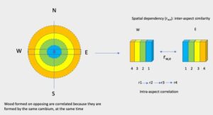
Heartwood color data represent a spatiotemporal repeated measurement on a tree. The properties on related trees and aspects are subject to correlations at any time due to shared genetic, physiological, and environmental effects. In addition, the wood properties of related trees at different points in time are also correlated due to the above factors. The long-short-axis data consists of two components representing spatial and temporal dependencies. By modelling the long-short axis data together, the dependency between the two aspects is accounted for in two ways: one for that between the aspects (i.e., purely spatial dependence) and the other for correlation within the long-short axis (i.e., purely temporal dependence). This modelling approach reveals the underlying process of heartwood color formation for the two aspects.
A general linear mixed model has the form (Laird and Ware 1982; Henderson 1984; Searle et al. 1992) as shown by Eq. 2:
y = Xβ + Zb + ε, (2)
b ~ N(0, G)
ε ~ N(0, R)
where y is the known vector of observations, β is a p x 1 vector of fixed effects with incidence matrix X, b is a q x 1 dimensional vector of random effects with corresponding design matrix Z, R is the variance-covariance matrix of errors and the random effects covariance matrix G. The expected value and variances are E[y] = Xβ, var[b] = G = and var[e] = R = for A the numerator relationship matrix and I an identity matrix.
Bivariate analysis
In the bivariate case, Eq. 2 was expanded to accommodate color trait values in the two aspects (stacking up the vectors), in such a way that β, b, and ε now contain the values for both radii (aspects).
 (3)
(3)
The symbol is the Kronecker product). The distribution of the random effects and error terms is assumed to be normal with mean zero and variance-covariance matrix,
 (4)
(4)
where and are the variances of the aspects 1 and 2, respectively, is the random treatment effects of covariance between aspects 1 and 2, and is the residual covariance between aspects 1 and 2. The nonzero covariances of random effects and error terms induce association between the responses. These represent the association of cambial evolution between the aspects and the evolution of cambial association over time, respectively.
Note that the two aspects are independent under joint normality if ![]() This implies there is no correlation at all between means of the trait in the two aspects.
This implies there is no correlation at all between means of the trait in the two aspects.
The Pearson correlation ( between the two aspects were estimated using the standard formula from the long-short axis variances and covariance components as,
 (5)
(5)

The coefficient of variation (CV) is given by,
CV = x 100 (6)
 The model (UN@AR (1)) adopted in this study assumes that the covariance matrix within a subject has the following structure:
 (7)
(7)
The UN takes care of the spatial correlation between the aspects, and AR(1) represents the correlation over time, which is assumed to be same for evolutions of color traits on the two aspects. The models in this paper were implemented in PROC MIXED from SAS 9.04 (SAS Institute, Cary NC) and solved using Restricted Maximum Likelihood (REML). In the modelling, the Kenward-Roger method (Kenward and Roger 1997) was used to determine degrees of freedom. The REML variance components were estimated. The homogeneity and normality of the residuals were checked to ensure that the assumptions were met by visual inspection, as per Schabenberger (2004). The F-test was used to determine the statistical significance of fixed effects (α = 0.05). Repeated measures ANOVA in which three types of heterogeneity (i.e., mean, variance, autocorrelation) were considered as follows,
Yijk = m + ai + rj + (a x r)ij + εijk (8)
where Yijk denotes individual color parameters (L*, a*, b*) for a tree k = 1, …, 3 at a distance from the pith (DFP) rj = 1, …, 10 along aspect ai = 1,2 at a given height level, m is the overall mean, and (a x r)ij is the interaction of aspect and distance from the pith. The experimental error is denoted by εijk. The spatial and temporal variations of the color parameter within and between trees was statistically evaluated using an ANOVA approach. Spatial heterogeneity was explained by aspect factor, while the distance from the pith factor accounted for temporal heterogeneity. After fitting the model, the bivariate data were simulated to create plots using the Eigen decomposition method. Aspect 2 (short axis) trait values were plotted against Aspect 1 (long axis). A regression line of aspect 2 against aspect 1, included in the bivariate variance structure for the evolution effects was drawn. The slope is given by Eq. 9
 (9)
(9)
RESULTS AND DISCUSSION
Table 1. Heartwood Color Parameters in the Long and Short Axis for Longitudinal Radial and Cross-sectional Surfaces (Average ± Standard Deviation)

Table 2. REML Estimates of the Model Parameters

Table 3. Pure Spatial Correlation (Simulated 5000 times)


Fig. 1. Scatter plot illustrating the association between Aspect 1 and Aspect 2 CIE L*, b*, and a* in the CS surface.

Fig. 2. Scatter plot illustrating the association between Aspect 1 and Aspect 2 CIE L*, b*, and a* in the LR surface.
Differences in Heartwood Color Between Surfaces and Aspects
The mean color values and their standard deviations are presented in Table 1. These values compare teak grown in Ghana (Derkyi et al. 2010) and grown elsewhere (Thulasidas et al. 2006; Moya and Calvo-Alvarado 2012). The two radii and surfaces were not identical, but the differences are neither significant statistically. The REML estimates of the variances of heartwood color traits for the two aspects are shown in Table 2. The variances for aspect 1 were almost as large as that for aspect 2 for L* in the LR surface, a* and b* in the CS surface. The covariance estimates were positive for all color parameters indicating the relationship between the aspects may be positive. Color can change more in one spatial dimension than the other, illustrating how plastic color traits are. Coefficients of variation (CV) were consistently larger for a*, particularly in the LR surface (>30%) and in the CS surface (about 18%). The color parameter L* showed the lowest CV (8% to 10%). The CV was about 9% to 14% for b*. The luminance index (L*) was higher on the fast-growing axis than on the slow-growing side of the LR surface, while the opposite was true on the CS. This is consistent with the assumption that fast-growing side may be lower in lignin content. Lignin is known to absorb visible light (Hon and Minemura 2001). Luminance variability (i.e., darkness or lightness) may be the primary source of variability in teak heartwood (Phelps et al. 1983). The color difference between the two radii can be attributed to the differential growth rate of cambium around the axes. This is consistent with Rink’s (1987) findings on black walnut that growth rate can affect heartwood color. The wood color difference between aspects on the LR surface was 0.46 and 2.88 in the CS. On the LR surface, the difference means little or no color difference, while on the CS a color difference is perceived rarely accepted (Buchelt and Wagenfuhr 2012). The wood color difference between the LR surface and CS surface was ∆E* = 4.65, which means the difference is significant (Buchelt and Wagenfuhr 2012). In this regard, teak heartwood surfaces may need to be graded in applications where a homogeneous color is desired. The color non-uniformity observed between the surfaces may be attributed to the pattern of wood cell arrangement in the two surfaces (Hon and Minemura 2001) and the variation in the quality and quantity of extractives (Keey 2005).
Spatial and Temporal Relationships
The association of traits in the two opposite sides is determined by correlations at two different levels: between- and within- aspect correlations. The underlying drivers of these correlations are physiological, genetic, chemical, and environmental mechanisms. The correlations between the aspects (i.e., purely spatial) were 0.18, 0.04, 0.33 for L*, a*, b*, respectively in the LR plane and 0.16, 0.22 and 0.36 for L*, a*, b*, respectively in the CS plane. These associations represent the mean values of the characteristics in the two aspects. These correlations were highly significant (Table 3). The b* color parameter showed a relatively stronger spatial correlation in both wood surfaces i.e., 0.33 and 0.36 for LR and CS. The positive correlation means that two characteristics are usually associated with each other, i.e., they move together. Also, the positive spatial correlation implies that the growth rate may not have an adverse impact on the color of the heartwood in teak. The contemporaneous correlations (i.e., purely temporal) or the correlations within an aspect measure the strength of the association between the change in one aspect between time lags and the corresponding change over the same time in the opposite aspect. The within-aspect correlations were 0.70, 0.67, 0.69 for L*, a*, b* in the LR plane and 0.71, 0.75 and 0.78 for L*, a*, b* in the CS plane. These correlations were highly significant. These correlations clarify the physiological basis for tree growth and development (Larson 1969; Fritts 1976). The wood color formed at the same presumed time on the opposite sides shows a stronger similarity or resemblance as opposed to wood color being poorly correlated with distance (between aspect). This may give an indication that the wood color can be controlled temporally in teak. The spatial and temporal autocorrelations indicate the spatiotemporal nature of wood formation. The two autocorrelations and their interactions show that the development of wood features is more complex. Spatial correlations can be employed to predict changes in color traits when selecting one aspect.
Measurement Associations of Heartwood Color Traits Between Aspects
The degree of association between two heartwood color parameters was measured by the regression coefficient. This expresses the change in trait 2 (aspect 2), in units of measurement, for each unit change in trait 1 (aspect 1). The estimated slopes were 0.15, 0.19, 0.30 for L*, a*, b*, respectively on the CS surface (see Figs. 1a, b, c). On the LR surface, the gradients were 0.17, 0.04, 0.26 for L*, a*, and b*, respectively (see Figs. 2a, b, c). The coefficients of determination were 3%, 0.15%, 10.7% for L*, a* and b*, respectively for LR surface. For the CS surface, coefficients of determination were 2.7%, 4.9%, 13.2% for L*, a*, and b*, respectively. The slope was consistently similar for L* on both surfaces. The color parameter b* recorded the highest slopes. This is likely to have resulted from the soil chemical constituents.
Effect of Growth Rate on Wood Color Parameters
To assess the effect of growth rate on color parameters, Type 3 fixed effects were applied, and the results are presented in Table 4. Differences between the aspects can be viewed as effects caused by differential growth rate (Taylor 1968; Williamson and Wiemann 2011). For all color parameters, the effect caused by aspect was not significant. This gives us an indication that growth rate may not be a statistically important factor in controlling teak heartwood color. Distance from the pith (DFP) was a significant factor for a* and b* in the LR surface and L* in the CS surface. The DFP as a factor controlling pith outwards variation of color parameters can be explained by the temporal degradation of previously formed extractives (Hillis 1987). There was no significant interaction between Aspect and DFP in all color traits in the two surfaces. This indicates that the differences among DFP can be modelled in the same way in two aspects.
Table 4. Tests of Fixed Effects in the Mixed Model Analysis of Variance for L*, a*, and b* in LR and CS Surfaces

Overall Findings
The answers to the two questions from this study are: (1) spatial correlation exists in heartwood color data from trees exhibiting eccentric growth and (2) spatial correlation was significant statistically but of low order (< r = 0.5) in all color parameters measured in the two surfaces. The bivariate analysis allows us to assess the variations and covariations in the two aspects jointly. In the present analysis, the variances for both aspects were non-zero for all traits (see Table 2). Variations in the color of the heartwood showed strong plasticity, implying that the color of the heartwood can change more in one aspect than in the other. The correlations between the two aspects were positive but of low order, less than 0.5 (Sokal and Oden 1978) for all color parameters in the two surfaces. This indicates that the color of the heartwood in teak can be affected by the environment and that they can have some degree of independent evolution that can be judged by the relatively lower slopes. This can be attributed to the differential rate of cambium production in the two aspects. The discs showed an average factor of 1.3 in eccentricity. Positive spatial autocorrelation can be attributed to microsite influences (Matern 1947). The microsite effect creates a positive spatial dependency because opposite sides of the same tree are subject to similar environmental conditions. From the purely spatial correlations, one can infer that the L* and a* color indices are more influenced by the heterogeneity of environmental conditions, which is consistent with Derkyi et al. (2010). The heartwood color parameter b* can show a stronger microsite effect than the others. This agrees with the results of Moya and Calvo-Alvarado (2012). Teak yellowness (b*) is reported to correlate positively with soil pH, calcium, magnesium but negatively with potassium, iron, and phosphorus (Derkyi et al. 2010; Moya and Calvo-Alvarado 2012), although the brightness parameter L* is known a better indicator of the durability of teakwood (Niamké et al. 2021). An interesting pattern was found in the brightness parameter; it was lower in the LR and CS surfaces for slow-growing and fast-growing sides, respectively. Because the color of the heartwood in teak is affected by secondary metabolites and the extractive chemical composition, it is expected that the proportion of the durability of the heartwood will be different even in the same tree at a specific height level. Also, some genes change gradually over time (Olesen 1978; Namkoong et al. 1988). In the present case, it can be assumed that ‘genetic’ correlations are due to pleiotropy rather than linkage equilibrium (Falconer 1952). Pleiotropy is simply the property of a gene, whereby it affects two or more traits, while linkage is more applicable to crosses between different strains (Falconer 1989), which should not be applicable in this study. The low “genetic” correlations imply that the heartwood color traits are to a great extent different and are probably controlled by different set of genes. When breeding for heartwood color in teak in Ghana, there may be a relatively higher tendency towards heritability in the b* color index. The positive correlations can be interpreted to mean that, at the spatial level, environmental conditions that enhance a color trait in one aspect enhance the opposite aspect. Heartwood color may be under heavy environmental control. The existence of significant spatial correlations raises an important problem with respect to the widely used traditional analysis method, namely regression analysis, which assumes error independence. This should be a warning to wood technologists who dismiss spatial and temporal dependencies as unworthy. It is important to realize that all assessments of wood quality are statistical and can be confusing unless the biological sources of variability are accounted for and explained (Larson 1969).
CONCLUSIONS
- A bivariate approach to test associations of wood traits measured over time from the same tree exhibiting eccentric growth could be a useful approach to clarify the variation and correlation structure of wood traits between the long-short axis at a time and over time.
- The bivariate modelling approach employed in this study is an attractive method of linking information both in space and time. Variations in spatial factors present no problems in this approach and could be a very useful follow up for detailed interpretation of wood formation pattern.
- The correlation between aspects and the error correlation reveals the underlying physiological mechanism in wood formation. The within-subject error correlation was relatively higher than the between-subject correlations. Considering both spatial and temporal autocorrelations can improve models and avoid biased results and misinterpretations.
- Heartwood color measured on opposite sides of the same tree shows a positive but low correlation (average r ~ 0.22). These results indicate that it may not be appropriate to use a core to determine heartwood color for the whole disc sampled at a specific height.
- The color parameter b* can have relatively low to moderate heritability and can be better than L* and a*. The presented results are preliminary and need to be evaluated in future studies with a larger sample size.
ACKNOWLEDGEMENTS
The first author was funded by MEXT for a PhD course at the Graduate School of Bioresource and Bioenvironmental Sciences, Kyushu University, Fukuoka, Japan.
REFERENCES CITED
Apertorgbor, M. M., and Roux, J. (2015). “Diseases of plantation forestry trees in southern Ghana,” Int. J. Phytopathol. 4, 5-13.
Bell, G., and Lechowicz, M. J. (1994). “Spatial heterogeneity at small scales and how plants respond to it,” in: Physiological Ecology, Exploitation of Environmental Heterogeneity by Plants, M. M. Caldwell, R.W. Pearcy (eds.), Academic Press.
Buchelt, B., and Wagenfuhr, A. (2012). “Evaluation of color differences on wood surfaces,” Eur. J. Wood Prod. 70, 389-391.
Burdon, R. D. (1977). “Genetic correlations for studying genotype-environmental interaction in forest tree breeding,” Silvae Genetica 26, 168-175.
Day, A.W. Jr., and Cote, A.C. (1965). Anatomy and ultrastructure of reaction wood, Syracuse University Press, Syracuse.
Derkyi, N. S. A., Bailleres, H., Chaix, G., Thevenon, M. F., Oteng-Amoako, A. A., and Adu-Bredu, S. (2010). “Color variation in teak (Tectona grandis) wood from plantations across ecological zones of Ghana,” Ghana J For 25, 40-49.
Gasparik, M., Gaff, M., Kačík, F., and Sikora, A. (2019). “Color and chemical changes in teak wood (Tectona grandis L. f.) and meranti wood after thermal treatment,” BioResources 14(2), 2667-2683. DOI: 10.15376/biores.14.2.2667-2683
Henderson, C. R. (1984). Applications of Linear Mixed Models in Animal Breeding, Guelph: University of Guelph, 426p.
Hillis, W. E. (1987). Heartwood and Tree Exudates, Springer-Verlag, Berlin, Germany.
Falconer, D. S. (1989). Introduction to Quantitative Genetics, John Wiley and Sons, New York.
Falconer, D. S. (1952). “The problem of environment and selection,” Amer. Nat. 86, 293-298.
FAO (2010). “Global forest resources assessment,” Country report, Ghana, Rome FRA 077.
Fayle, D. C. F. (1973). “Patterns of annual xylem increment integrated by contour presentation,” Can. J. For. Res. 3, 105-111.
Friml, J. (2003). “Auxin transport – shaping the plant,” Current Opinion in Plant Biology 6, 7-12.
Fritts, H. C. (1976). Tree Rings and Climate, Academic Press, London, U.K.
Hon, D. N., and Minemura, N. (2001). “Color and discoloration,” in: Wood and Cellulosic Chemistry, D. N. S. Hon, N. Shiraishi (eds.), Marcel Dekker, New York.
Keey, R. (2005). “Colour development on drying,” Maderas. Ciencia y tecnologica 7, 3–16.
Kenward, M.G., and Roger, J.H. (1997). “Small sample inference for fixed effects from restricted maximum likelihood,” Biometrics 53(3), 983–997.
Klumpers, J., Janin, G., Becker, M., and Levy, G. (1993). “The influences of age, extractive content and soil water on wood color in oak: the possible genetic determination of wood color,” Ann Sci For 50(Suppl. 1), 403s– 409s.
Lande, R. (1979). “Quantitative genetic analysis of multivariate evolution applied to brain: body size allometry,” Evolution 33, 402-416.
Lande, R., and Arnold, S. J. (1983). “The measurement of selection on correlated characters,” Evolution 37, 1210-1226.
Larson, P.R. (1964). “Some indirect effects of environment on wood formation,” in: The Formation of Wood in Forest Trees, M. H. Zimmermann (ed.), Academic Press, New York.
Larson, P. R. (1969). “Wood formation and the concept of wood quality,” Yale Univ. For. Bull. 74, 1-54.
Laird, N. N., and Ware, J. H. (1982). “Random effects models for longitudinal data,” Biometrics 38, 963-974.
Lukmandaru, G., and Takahashi, K. (2009). “Radial variation of quinones in plantation teak (Tectona grandis, L.f.),” Ann For Sci 66, 605.
Matern, B. (1947). “Metoder att upskatta noggrannheten vid linjeoch provytetaxering (Methods of estimating the accuracy of line and sample plot surveys),” Medd. Fran Statens Skogsforskninsinstitut, Nr. 1, p. 36 (in Swedish with English summary).
Moya, R., Bond, B., and Quesada, H. (2014). “Review of heartwood properties of Tectona grandis trees from fast-growth plantations,” Wood Sci Technol 48, 411-433.
Namkoong, G., Kang, H. C., and Brouard, J. S. (1988). Tree Breeding Principles and Strategies, Springer-Verlag, New York.
Niamké, F. B., Amusant, N., Augustin, A. A., and Chaix, G. (2021). “Teakwood chemistry and natural durability,” in: The Teak Genome. Compendium of Plant Genome, Y. Ramasamy, E. Galeano, T. T. Win (eds.), Springer, Cham.
Olesen, P. O. (1978). “On cyclophysis and topophysis,” Silvae Genetica 27, 173-178.
Phelps, J. E., McGinnes, E. A., Garnet, H. E. J., and Cox, G. S. (1983). “Growth quality evaluation of black walnut wood. Part III. Color analysis of veneer produced at different sites,” Wood Fiber Sci 15, 177-185.
Pruyn, M. L., Ewers, B. J., and Telewski, F. W. (2000). “Thigmomorphogenesis: changes in the morphology and mechanical properties of two Populus hybrids in response to mechanical perturbation,” Tree Physiol 20, 535-540.
Rink, G. (1987). “Heartwood color and quantity variation in young black walnut progeny test,” Wood Fiber Sci 19(1), 93-100.
Rudman, P., and Gay, F. J. (1961). “The causes of natural durability in timber part VI. Measurement of anti-termite properties of anthraquinones from Tectona grandis L.f. by rapid semi-micro method,” Holzforschung 117.
SAS Institute Inc. (2004). SAS Online Doc® 9.1.3. SAS Institute Inc., Cary, North Carolina.
Savidge, R. A. (2003). “Tree growth and wood quality,” in: Wood Quality and Its Biological Basis, J. R. Barnett, G. Jeronimidis (eds.), Blackwell Scientific, Oxford.
Searle, S. R., Casella, G., and McCulloch, C. E. (1992). Variance Components, John Wiley, New York.
Schabenberger, O. (2004). “Mixed model influence diagnostics,” Proceedings of the Twenty-Ninth Annual SAS® Users Group International (SUGI) Conference, pp. 189-29. SAS Institute Inc., Cary, North Carolina.
Sokal, R. R., and Oden, N. L. (1978). “Spatial autocorrelation in biology 2. Some biological implications and four applications of evolutionary and ecological interest,” Biological Journal of the Linnean Society 10, 228-249
Sumthong, P., Damvelg, R. A., Choi, Y.H., Arentshorst, M., Ram, A. F., Van den Hondel, C. A. M. J. J., and Verpoorte, R. (2006). “Activity of quinones from teak (Tectona grandis) on fungal cell wall stress,” Planta Med. 72, 943-944.
TAPPI T527 om-94. (1994). “Color of paper and paper board (d/0o geometry),” Tappi Press, Atlanta, GA.
Taylor, F. W. (1968). “Specific gravity differences within and among yellow-poplar trees,” Forest Products J 18(3), 75-81.
Thulasidas, P. K., Bhat, K. M., and Okuyama, T. (2006). “Heartwood color variation in home garden teak (Tectona grandis) from wet and dry localities of Kerala, India,” Journal of Tropical Forest Science 18(1), 51-54.
Via, S. (1984). “The quantitative genetics of polyphagy in an insect herbivore. II. Genetic correlations in larval performance within and among host plants,” Evolution 38, 896-905.
Via, S. (1991). “The genetic structure of host plant adaptation in a spatial patchwork: demographic variability among reciprocally transplanted pea aphid clones,” Evolution 45, 827-852.
Williamson, G. B., and Wiemann, M. C. (2011). “Age versus size determination of radial variation in wood specific gravity: Lessons from eccentrics,” Trees 25, 585-591.
Article submitted: July 11, 2022; Peer review completed: September 11, 2022; Revisions accepted: September 12, 2022; Published: September 19, 2022.
DOI: 10.15376/biores.17.4.6178-6190