Accelerated air-coupled ultrasound imaging of wood using compressed sensing

Abstract

Air-coupled ultrasound has shown excellent sensitivity and specificity for the nondestructive imaging of wood-based material. However, it is time-consuming, due to the high scanning density limited by the Nyquist law. This study investigated the feasibility of applying compressed sensing techniques to air-coupled ultrasound imaging, aiming to reduce the number of scanning lines and then accelerate the imaging. Firstly, an undersampled scanning strategy specified by a random binary matrix was proposed to address the limitation of the compressed sensing framework. The undersampled scanning can be easily implemented, while only minor modification was required for the existing imaging system. Then, discrete cosine transform was selected experimentally as the representation basis. Finally, orthogonal matching pursuit algorithm was utilized to reconstruct the wood images. Experiments on three real air-coupled ultrasound images indicated the potential of the present method to accelerate air-coupled ultrasound imaging of wood. The same quality of ACU images can be obtained with scanning time cut in half.

Full Article

Accelerated Air-coupled Ultrasound Imaging of Wood Using Compressed Sensing

Yiming Fang,^a,b Zhixiong Lu,^a,* Lujun Lin,^b Hailin Feng,^b and Junjie Chang ^c

Air-coupled ultrasound has shown excellent sensitivity and specificity for the nondestructive imaging of wood-based material. However, it is time-consuming, due to the high scanning density limited by the Nyquist law. This study investigated the feasibility of applying compressed sensing techniques to air-coupled ultrasound imaging, aiming to reduce the number of scanning lines and then accelerate the imaging. Firstly, an undersampled scanning strategy specified by a random binary matrix was proposed to address the limitation of the compressed sensing framework. The undersampled scanning can be easily implemented, while only minor modification was required for the existing imaging system. Then, discrete cosine transform was selected experimentally as the representation basis. Finally, orthogonal matching pursuit algorithm was utilized to reconstruct the wood images. Experiments on three real air-coupled ultrasound images indicated the potential of the present method to accelerate air-coupled ultrasound imaging of wood. The same quality of ACU images can be obtained with scanning time cut in half.

Keywords:  Air-coupled ultrasound; C-scan; Imaging of wood; Compressed sensing; Undersampled scanning trajectory 

Contact information:  a:  College of Engineering, Nanjing Agricultural University, No. 40, Dianjiangtai Road, Nanjing 210031, China; b: College of Information Engineering, Zhejiang A & F University, No. 88, North Huancheng Road, Lin’an, Hangzhou 311300, China; c: Japan Probe Co., Ltd., Yokohama 2320033, Japan; *Corresponding author: luzx@njau.edu.cn

INTRODUCTION

After considerable development, air-coupled ultrasound (ACU) C-scan imaging has found a greater number of applications in the inspection of wood and wood composites. The work by Gan et al. (2005) demonstrated ACU’s capacity for high-resolution imaging. Ring density and the presence of micro-cracks can be imaged. Fleming et al. (2005) investigated the presence of insects inside the solid wood packing materials. The presence and movement of beetle larva were identified when the larva was placed on the wood. Studies on the bonding assessment of glued timber and microstructure classification in particleboards were also reported. The geometry of the artificial defects of glued timber was presented clearly. The density distributions and particle profiles in particleboards were also obtained using a non-linear model (Hilbers et al. 2012a,b; Sanabria 2012; Sanabria et al. 2013). In an earlier paper the authors reported using the ACU C-scan technique to test Metasequoia glyptostroboides boards. Knot, hole, heartwood, and sapwood were shown clearly in the obtained images. Information regarding position, shape, and size can be extracted easily (Fang et al. 2015).

Although ACU C-scan imaging can be used to form images under laboratory conditions, there is a problem that must be overcome. To acquire adequate information and reconstruct high-quality images, it is desirable to scan the wood at sufficiently high sampling densities. Under the constraints of large measurement numbers and low motor speed, ACU C-scan imaging is considerably time-consuming (Blomme et al. 2014). A common approach is to decrease the sampling density, which could shorten the scanning time. Unfortunately, the decreased sampling density frequently results in a poor image, and it even causes the image to suffer from aliasing due to the restriction of the Nyquist-Shannon sampling theorem. Therefore, only a small number of successful attempts with industrial relevance have been mentioned in the literature until now (Chimenti 2014).

During past decades, efforts have been made to address this problem. A multi-channel system was introduced to achieve a high scanning speed. Strycek and Loertscher (2000) developed an eight-channel Flatbed Scanner, which provides the capability of scanning at a rate of 350 square meters/hour. Blomme et al. (2014) reported another twelve-channel scanning system for scanning large material areas. However, the multi-channel system tends to result in higher cost because more transducers have to be used. Moreover, the cross-coupling of signals poses a formidable challenge to the realization of inspection. Ultrasound waves propagate to the adjacent transducers as guided waves, as well as to the matched transducer. It becomes very difficult to separate unwanted signals from the useful ones (Strycek and Loertscher 2000).

Recently, compressed sensing (CS), proposed by Donoho (2006) and Candès et al. (2006), shows high promise for recovering signals (or images) with excellent accuracy while acquiring only a small fraction of them. CS has inspired a number of efficient new designs for image acquisition, including hyperspectral imaging (Jia et al. 2015), synthetic aperture radar (SAR) imaging (Yang et al. 2013), electron paramagnetic resonance imaging (EPRI) (Johnson et al. 2014), etc. Previous studies indicate that using the CS approach in ACU C-scan imaging may become attractive and reduce the scanning duration significantly.

However, the conditions under which CS performs well are not necessarily met in practice. Under the standard CS framework, each measurement corresponds to a linear projection of multiple measurements. It is an inspiring and instructive idea because the linear projection produces sufficient incoherence with the representation basis and stable foundation for CS application. However, it is indeed impractical for the ACU imaging system. The scanning is conventionally implemented along parallel, equally spaced lines in the Cartesian coordinate system. The linear projection is hardly possible to be implemented. Furthermore, to reconstruct the desired image, a good representation basis is required to represent the undersampled data sparsely in the transform domain. Unfortunately, it is not immediately clear how to find the representation basis. There is no systematic way of selecting such a matrix. It is usually done through trials and experience (Quer et al. 2009). In the subsequent sections, the methods for overcoming the practical constraints are addressed.

Related CS Theory

Compressed sensing is based upon an assumption that the sparse signals can be reconstructed exactly from many fewer measurements than traditionally believed necessary. Consider a discrete-time signal x, which can be viewed as an  column vector with elementsWith an orthonormal asis

matrix, the signal x can be represented in the transform domain as follows (Eq. 1),

where s is the column vector of weighting confidents  If only K of the confidents s_i in Eq. 1 are nonzero and, signal x can be considered to be sufficiently sparse in the transform domain. Then the exact recovery of x is possible.

In the CS framework, it is assumed that the signal x is not measured directly. Rather, the linear projections of the original signal onto another suitably chosen matrixare measured (Eq. 2),

where y is the measurement vector and has a length of M. is an  matrix which is usually called the measurement matrix.

The signal recovery problem is transferred to reconstruct s (and thus x) from the given measurement vector y and known matrices and . Since , there are infinitely many reconstructed  that satisfy Eq. 2. It has been proposed in the literature (Baraniuk 2007) that with the smallest l₀-norm can be considered as the desired signal due to the sparsity mentioned above. Then the reconstruction can be obtained by solving the following constrained optimization problem (Eq. 3):

            Unfortunately, solving Eq. 3 is both numerically unstable and Np-complete. Subsequently, it was suggested that the minimum l₁-norm can be employed as an alternative to the l₀-norm (Baraniuk 2007). This means that  can be reconstructed by the convex optimization method (Eq. 4):

            To illustrate the approach with a practical example, a continuous signal,

was considered. Figure 1(a) shows the waveform in time domain. The duration is 320 ms. A discrete vector x with a length of 256 can be obtained while sampling the continuous signal with a sampling frequency of 800 Hz. According to the Fourier transform theory, the vector x can be expressed as product of the Discrete Fourier Transform (DFT) matrix and the confident vector s (Eq. 5),

Where 

Consider an 256*64 matrix which contains random values drawn from the Gaussian distribution. According to Eq. 2, a measurement vector y can be obtained by multiplying the discrete signal x with the random matrixEq. (6),

Where  

Obviously, the elements of measurement vector y are not extracted directly from the discrete signal x. Rather, the elements are obtained from a projection of x onto the Gaussian matrix. Figure 1 (b) shows the result of the projection.

By solving the convex optimization problem described in Eq. 4, the reconstructed coefficient vector  can be computed. Finally, the reconstructed signal can be obtained by a DFT transform according to Eq. 5. Figure 1(c) shows the reconstructed result. It is obvious that signal was reconstructed with high accuracy.

Fig. 1. Schematic illustration of undersampled measurement and signal reconstruction using the CS approach: (a) A simulation signal; (b) result of undersampled measuring; (c) Recovered signal

ACU C-SCAN Imaging Based on CS

Scanning Trajectory

Figure 2(a) illustrates the conventional scanning trajectory in the ACU C-scan imaging system (Sanabria et al. 2011). The transducer-pair is moved along the parallel, equally spaced lines. This scheme produces a two-dimensional matrix (y), which is frequently displayed with an image. The color or gray level of the image’s pixel is determined by the amplitude or time-of-flight of the through-transmitted sound. The number of scanning lines (N) determines the scanning time and is limited by the Nyquist frequency. The scanning can be mathematically expressed as , as shown in Fig. 2(b). Obviously, it looks similar to Eq. 2, but here is a unit matrix of size N rather than the random matrix.

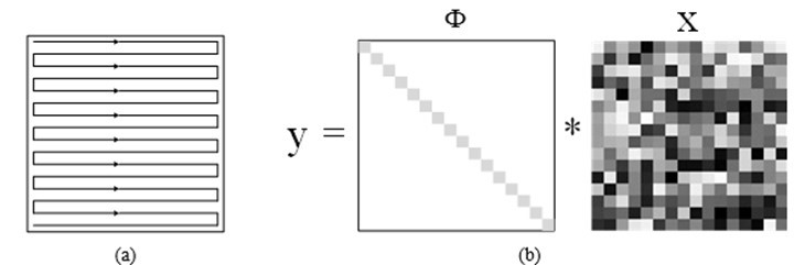
Fig. 2. Conventional Nyquist scanning trajectory in the ACU C-scan imaging system: (a) Graphic depiction; (b) Mathematical depiction

As mentioned above, the purpose of this work is to reconstruct images with a fraction of the scanning and then reduce the overall scanning time. This is a typical application of CS because the size of measurement matrix (M*N) is smaller than that of the square matrix (N*N).  However, it is hard to implement the linear projection under standard CS framework in the C-scanning system. Lustig et al. (2008) proposed a simple but indeed practical method. Figure 3(a) illustrates the undersampled scanning trajectory. Entire scanning lines (dash lines) were dropped randomly from an existing complete grid. The transducer-pair only needed to walk along the solid lines. It is very convenient to implement a scan in this way since the implementation requires only minor modifications to the existing ACU C-scanning imaging system.

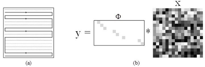
Fig. 3. Undersampled scanning trajectory for high-speed ACU imaging; (a) Graphic depiction; (b) Mathematical depiction

Likewise, the undersampled scanning can be expressed mathematically as. The matrixhere specifies a scanning scheduling policy shown in Fig. 3 (a). The element “1” in the i^th array indicates that the i^th line of the grid should be scanned. Generally, “1” appears along a diagonal line because it is easier to implement if the movement is in a single direction during the scanning from top to bottom. Let M denote the total number of rows of . The sampling ratio can be defined as M/N. It takes a shorter time to implement a scanning if the sampling ratio is smaller.

Although the leakage of information is inevitably caused by undersampled scanning, it is widely accepted that the entire image can be exactly reconstructed if “1” appears randomly and its index follows the Gaussian distribution (Eldar and Kutyniok 2012).

Sparse Representation and Reconstruction

A variety of linear transforms have been used as the representation basis. In this work, three well-known transformations were considered. This selection was determined by previous papers based on their prominence in other CS applications. The three bases were discrete Fourier transform (DFT) basis, discrete cosine transform (DCT) basis, and discrete wavelet transform (DWT) basis.

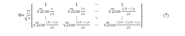
The DFT matrix has been introduced in Eq. 5. The form of DCT used here was type-II, which is the most commonly used. The DCT matrix is as follows Eq. 7:

As the representation in the DWT domain relies heavily on the selection of the wavelet basis and the decision of the wavelet decomposing scale, Schmale et al. (2013) examined 15 different mother wavelets. The results indicated that symlet 8 provided the lowest number of significant coefficients and yielded the best sparsity. Thus, symlet 8 was selected in the following discussion.

The last factor to determine for CS is the best optimization algorithm for solving the -norm minimization problem. Assume y_i is the i^th column of the undersampled data y. The coefficient vector  can be obtained by solving Eq. 4 with known matrix and Then the i^th column  of the ideal image can be reconstructed from  with a linear transform illustrated in Eq.1.

There are quite a few typical algorithms, such as basis pursuit (BP), matching pursuit (MP), and orthogonal matching pursuit (OMP). This paper considered the OMP algorithm, which has been widely used for this purpose. An  is firstly defined as sensing matrix for the convenience of description. The flow chart of OMP algorithm is schematically shown in Fig.4  (Tropp and Gilbert 2007).

In initialization, the iteration counter is set equal to 1, the initial residual r₀ is assigned to the input vector y_i, and the index setis assigned to an empty set. Then the matrix of chosen atoms  is also an empty set.

The task of atom searching is to find the indexthat solves the easy optimization problem. In this step, the inner product between the column vectors of the sensing matrixare computed. Maximizing the product leads to the optimal choice, which is given here as Eq. 8,

Where  

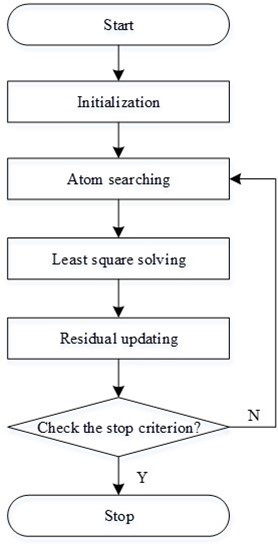
Fig. 4. Flow chart of the OMP algorithm

Subsequently, the index  is added to the index set  and the matrix of chosen atoms is updated as.

The step of least square solving is aiming for computing the new estimation.  The new estimation can be obtained by minimizing of , and the residual updating step is performed as represented by Eq. 9,

where y_i is the i^th column of the undersampled data. It is fed into the OMP algorithm when it is called at the  y_i time.

Finally, t is increased with the increment of 1. If  is smaller than the given sparsity level of the input y_i, the process returns to the step of atom searching. Otherwise, the iteration is stopped and the output estimation is  According to Eq.1, the i^th column of the ideal image,  can be computed. After the OMP algorithm is run for N times, the ideal image is reconstructed.

EXPERIMENTAL

Three Metasequoia glyptostroboides boards were used. These boards had a thickness of 8 mm. One board had a sound condition. The grain can be seen clearly. Another board had a decay knot. A part of the knot was seriously deteriorated and had fallen off. In the last board, two holes with diameters of 4 mm and 5 mm were drilled to simulate the insect holes. Figure 5 displays photos of the wooden samples used in the experiment.

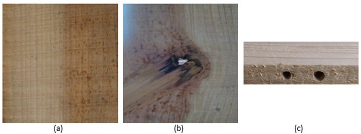
Fig. 5. Photos of the Metasequoia glyptostroboides boards

A non-contact ACU inspection system (Model: NAUT 21, Manufacturer: Japan Probe Co., Ltd., Japan), as shown in Fig. 6, was utilized in the experiment. The transducers had central frequency of 400 KHz. The diameter of focal spot was 2 mm. Burst waves including five rectangular pulses were generated, amplified to 300 Vpp amplitude, and fed into the transmitter transducer. Received signals were filtered and amplified 70 dB with a preamplifier.  Images were generated from the peak voltage measurement for each A-scan.

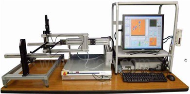
Fig. 6. The ACU C-scan imaging system used in this work

The samples were fully scanned with an increment of 0.5 mm. The fully-scanned data were then trimmed to images with size of 256 × 256 pixels for the convenience of experiment. Figure 7 shows theses chosen images. The image in Fig. 7(a) illustrates the wood grain arrangement. Figure 7(b) shows the image of a decay knot. The circular dark region corresponded with the seriously deteriorated part of the knot. Figure 7(c) is an image of a sample with two drilled holes. The holes were depicted with a darker color.

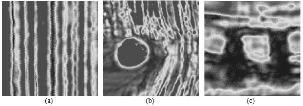
Fig. 7. Real ACU images of Metasequoia glyptostroboides boards utilized in this work. Their sizes are 256 × 256 pixels: (a) grain image; (b) knot image; (c) and drilled hole image

Apart from visual comparison, the Peak Signal-to-Noise Ratio (PSNR) was used to measure the quality of reconstruction. Generally, a higher PSNR indicates that the reconstruction is of higher quality. PSNR was calculated using Eq. 10,

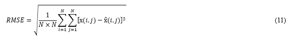
where  is the maximum gray level of pixels. As for the 8-bit image format which was used in this work,  is equal to 255. RMSE denotes the root-mean-square error between the original image (x) and the reconstructed image ( )(Eq. 11):

RESULTS AND DISCUSSION

Reconstructing Images from the Undersampled Data with DCT Basis

The proposed method was applied to images shown in Fig. 7 to evaluate the effectiveness in the Matlab environment. At first, the undersampled scanning was simulated mathematically. A random binary matrix  was generated with lines of 128 to achieve the sampling ratio of 50%. There was only one element of “1” appearing in each row of the matrix. The indexes of “1” in the whole matrix obeyed Gaussian distribute and were sorted to achieve high suitability for the mechanical system of the existing C-scanner. The matrixwas applied to the three fully-scanned images shown in Fig. 7 to simulate the undersampled scanning.

Figure 8 shows the results of undersampled scanning. It can be seen that the width of the images remained unchanged whereas the height was changed to half of those of the fully-scanned image.

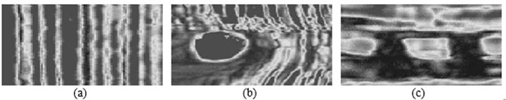
 Fig. 8. Results of undersampled scanning at 50% sampling ratio (128 × 256 pixels): (a) grain image; (b) knot image; (c) and hole image

Subsequently, each undersampled image was treated as 256 vectors. The vectors were fed into the OMP optimization process with DCT matrix as the representation basis.  After the OMP algorithm was run for 256 times, an ideal images can be obtained. Figure 9 shows the reconstructed results. As expected, the images can be effectively reconstructed and the reconstructions were very close to the original images. The grain, knot, and hole can still be clearly seen in the reconstructed images. It can be concluded that the same quality of ACU images can be obtained with scanning time cut in half.

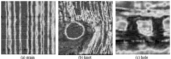
 Fig. 9. Reconstructed images (256 × 256 pixels) at 50% sampling ratio with DCT basis: (a) grain image; (b) knot image; (c) and hole image

Comparisons of the Representation Bases

The experiments were also conducted with DFT basis and DWT basis to study their performance. Figure 10 and Fig.11 show the reconstructed results.

 Fig. 10. Reconstructed images (256 × 256 pixels) at 50% sampling ratio with DFT basis: (a) grain image; (b) knot image; (c) and hole image

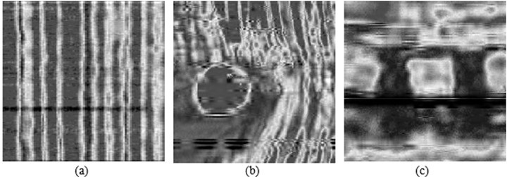
 Fig. 11. Reconstructed images (256 × 256 pixels) at 50% sampling ratio with DWT basis: (a) grain image; (b) knot image; (c) and hole image

The sampling ratio was also 50%. Compared with the images shown in Fig. 9, it can be seen that the DCT basis always obtained the best visual effects on all ACU images. The DWT basis was far worse than the others.

To evaluate the reconstruction performance of the three representation bases furtherly, a set of experiment were run by increasing the sampling ratio from 20% to 90%. The average PSNR (left) and standard deviation (right) are exhibited in Fig. 12. They were computed with the results of 100 realizations.

Overall, all the representation bases showed very similar performance. Along with the increase of the sampling ratio from 20% to 90%, the average PSNR increased considerably. These observation indicated that the sampling ratio plays a crucial role in determining the reconstruction quality. A larger sampling ratio also leads to higher measurement cost.

It also can be observed that the DCT basis is capable of producing the best performance. For all the three image reconstructions, it achieved a bigger PSNR in nearly every experiment compared to the DFT basis and DWT basis. This result agrees with that of the visual comparison.

And what’s more, the standard deviations of the DCT basis were low and fluctuated gently compared with the DFT basis and the DWT basis. This meant the DCT basis is insensitive to the randomness of the sampling trajectory. It is a more robust representation method than other two bases.

Comparison with the Standard CS

For comparison, the standard CS was run with the fully-scanned images, although it is not practical for this problem.

The major difference lies in the measurement matrix . Instead of the random binary matrix, the measurement matrix  used in this experiment was the Gaussian matrix generated by the MATLAB code randn.m.

Under the Gaussian matrix, each measurement corresponds with a linear projection of multiple pixels. Figure 13 illustrates the performance of standard CS. The sampling ratio ranged from 20% to 90% and the results were calculated with 100 repetitions.

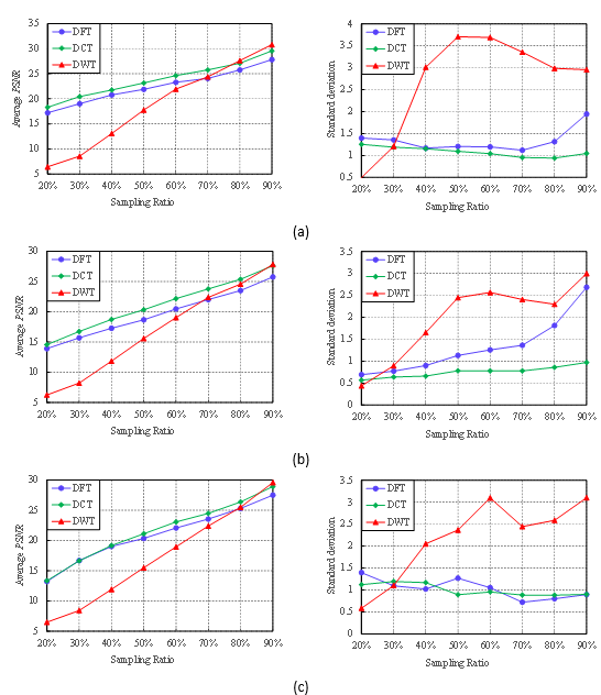
Fig. 12. Performance of three representation bases at different sampling ratios: (a) grain image; (b) knot image; (c) and hole image

Compared with Fig. 12, it can be seen that the DCT basis behaved similarly as the preceding experiments. In the same setting, the ranges of average PSNR for three images were 17.56 ~ 30, 12.57 ~ 29.38 and 13.93 ~ 28.52, respectively. The standard deviations fluctuated near 1. This means that the DCT basis can achieve the same successes under the proposed method as the standard CS in spite of the considerable difference between the two measurement matrixes. But the average PSNR and the standard deviation corresponding to the DWT basis changed considerably. When sampling ratio ranged from 40% to 90%, the DWT basis can achieve the best performance. The average PSNR was the largest one than those of the other two bases, whereas the standard deviation was the smallest. However, at the sampling ratios of 20% and 30%, the DWT basis was still the worst one. The average PSNR dropped rapidly while the standard deviation increased sharply. It is worth noting that the cases at low sampling ratios tend to receive more attention in high-speed ACU imaging systems because the scanning times can be reduced to a greater degree. It can be concluded that the DCT basis is a better choice in this problem considering the imaging speed.

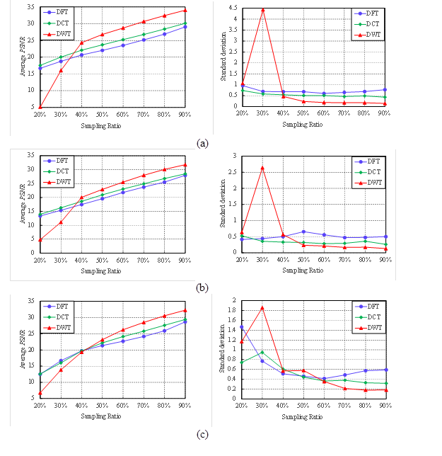
Fig. 13. Reconstruction performance of the standard CS: (a) grain image; (b) knot image; (c) and hole image         

CONCLUSIONS

1. By using the CS-based approach, ACU imaging of wood can be accelerated significantly. Compared with the conventional C-scanning, the proposed method can achieve approximately the same performance while taking only half of the time.
2. The proposed scanning trajectory is particularly appealing because the undersampled scanning is extremely easy to implement with only minor modification to the existing ACU imaging system.
3. Accuracy of reconstruction is sensitive to the sparse basis that is used to represent the wood images in the transform domain. Compared with the DFT basis and the DWT basis, the DCT basis achieved the highest PSNR. A better representation method might produce a better reconstruction performance. Further study is needed to confirm this.

ACKNOWLEDGMENTS

The authors acknowledge the support of the Natural Science Foundation of China (Nos. 61302185, 61272313, and 61472368) and the Zhejiang Provincial Science and Technology Project (Nos. 2013C31018 and LQ14F020014). The authors also gratefully acknowledge the financial support of the Zhejiang Provincial Key Laboratory of Forestry Intelligent Monitoring and Information Technology (No. 100151402).

REFERENCES CITED

Baraniuk, R. G. (2007). “Compressive sensing,” IEEE Signal Processing Magazine 24(4), 118-121. DOI: 10.1109/MSP.2007.4286571

Blomme, E., Naert, H., Bilcke, M., Lust, P., Delrue, S., and Van Den Abeele, K. (2014). “High speed air-coupled ultrasonic multichannel system,” in: Proceedings of the 2014 Forum Acusticum, Krakow, Poland. (http://www.fa2014.agh.edu.pl/fa2014_cd/article/SS/SS19_3.pdf).

Candès, E. J., Romberg, J., and Tao, T. (2006). “Robust uncertainty principles: Exact signal reconstruction from highly incomplete frequency information,” IEEE Transactions on Information Theory 52(2), 489-509. DOI: 10.1109/TIT.2005.862083

Chimenti, D. (2014). “Review of air-coupled ultrasonic materials characterization,” Ultrasonics 54(7), 1804-1816. DOI: 10.1016/j.ultras.2014.02.006

Donoho, D. L. (2006). “Compressed sensing,” IEEE Transactions on Information Theory 52(4), 1289-1306. DOI: 10.1109/TIT.2006.871582

Eldar, Y. C., and Kutyniok, G. (2012). Compressed Sensing: Theory and Applications, Cambridge University Press, Cambridge, UK

Fang, Y., Lu, Z., Lin, L., and Feng, H. (2015). “Application of air-coupled ultrasonic imaging technique for nondestructive testing of solid wood board,” ICIC Express Letters, Part B: Applications 6(10), 2773-2778.

Fleming, M. R., Bhardwaj, M. C., Janowiak, J. J., Shield, J. E., Roy, R., Agrawal, D. K., Bauer, L. S., Miller, D. L., and Hoover, K. (2005). “Noncontact ultrasound detection of exotic insects in wood packing materials,” Forest Products Journal 55(6), 33-37.

Gan, T. H., Hutchins, D. A., Green, R. J., Andrews, M. K., and Harris, P. D. (2005). “Noncontact, high-resolution ultrasonic imaging of wood samples using coded chirp waveforms,” IEEE Transactions on Ultrasonics, Ferroelectrics and Frequency Control 52(2), 280-288. DOI: 10.1109/TUFFC.2005.1406553

Hilbers, U., Neuenschwander, J., Hasener, J., Sanabria, S. J., Niemz, P., and Thoemen, H. (2012a). “Observation of interference effects in air-coupled ultrasonic inspection of wood-based panels,” Wood Science and Technology 46(9), 979-990. DOI: 10.1007/s00226-011-0460-9

Hilbers, U., Thoemen, H., Hasener, J., and Fruehwald, A. (2012b). “Effects of panel density and particle type on the ultrasonic transmission through wood-based panels,” Wood Science and Technology 46(4), 685-698. DOI: 10.1007/s00226-011-0436-9

Jia, Y., Feng, Y., and Wang, Z. (2015). “Reconstructing hyperspectral images from compressive sensors via exploiting multiple priors,” Spectroscopy Letters 48(1), 22-26. DOI: 10.1080/00387010.2013.850727

Johnson, D. H., Ahmad, R., He, G., Samouilov, A., and Zweier, J. L. (2014). “Compressed sensing of spatial electron paramagnetic resonance imaging,” Magnetic Resonance in Medicine 72(3), 893-901. DOI: 10.1002/mrm.24966

Lustig, M., Donoho, D. L., Santos, J. M., and Pauly, J. M. (2008). “Compressed sensing MRI,” IEEE Signal Processing Magazine 25(2), 72-82. DOI: 10.1109/MSP.2007.914728

Quer, G., Masiero, R., Munaretto, D., Rossi, M., Widmer, J., and Zorzi, M. (2009). “On the interplay between routing and signal representation for Compressive Sensing in wireless sensor networks,” in: Proceedings of 2009 Information Theory and Applications Workshop, San Diego, CA, 206-215. DOI: 10.1109/ITA.2009.5044947

Sanabria, S. J. (2012). “Air-coupled ultrasound propagation and novel non-destructive bonding quality assessment of timber composites,” Ph.D. Thesis, ETH Zurich, Switzerland.

Sanabria, S. J., Hilbers, U., Neuenschwander, J., Niemz, P., Sennhauser, U., Thömen, H., and Wenker, J. L. (2013). “Modeling and prediction of density distribution and microstructure in particleboards from acoustic properties by correlation of non-contact high-resolution pulsed air-coupled ultrasound and X-ray images,” Ultrasonics 53(1), 157-170. DOI: 10.1016/j.ultras.2012.05.004

Sanabria, S. J., Mueller, C., Neuenschwander, J., Niemz, P., and Sennhauser, U. (2011). “Air-coupled ultrasound as an accurate and reproducible method for bonding assessment of glued timber,” Wood Science and Technology 45(4), 645-659. DOI: 10.1007/s00226-010-0357-z

Schmale, S., Knoop, B., Hoeffmann, J., Peters-Drolshagen, D., and Paul, S. (2013). “Joint compression of neural action potentials and local field potentials,” 2013 Asilomar Conference on Signals, Systems and Computers, Pacific Grove, CA, 1823-1827. DOI: 10.1109/ACSSC.2013.6810617

Strycek, J., and Loertscher, H. (2000). “High speed large area scanning using air-coupled ultrasound,” in: Proceedings of the 15^th World Conference on Nondestructive Testing, Roma. (http://www.ndt.net/article/wcndt00/papers/idn209/idn209.htm)

Tropp, J., and Gilbert, A. C. (2007). “Signal recovery from random measurements via orthogonal matching pursuit,” IEEE Transactions on Information Theory 53(12), 4655-4666. DOI: 10.1109/TIT.2007.909108

Yang, J., Thompson, J., Huang, X., Jin, T., and Zhou, Z. (2013). “Random-frequency SAR imaging based on compressed sensing,” IEEE Transactions on Geoscience and Remote Sensing 51(2), 983-994. DOI: 10.1109/TGRS.2012.2204891

Article submitted: July 26, 2015; Peer review completed: October 24, 2015; Revised version received and accepted: November 22, 2015; Published: December 3, 2015.

DOI: 10.15376/biores.11.1.1015-1030