Geospatial economics of the woody biomass supply in Kansas

Khaliukova, O., Paull, D., Lewis-Gonzales, S. L., André, N., Biles, L. E., Young, T. M., and Perdue, J. H. (2017). "Geospatial economics of the woody biomass supply in Kansas - A case study," BioRes. 12(1), 960-980.

Abstract

This research assessed the geospatial supply of cellulosic feedstocks for potential mill sites in Kansas (KS), with procurement zones extending to Arkansas (AR), Iowa (IA), Missouri (MO), Oklahoma (OK), and Nebraska (NE). A web-based modeling system, the Kansas Biomass Supply Assessment Tool, was developed to identify least-cost sourcing areas for logging residues and upland hardwood roundwood biomass feedstocks. Geospatial boundaries were used according to the 5-digit zip code tabulation area (ZCTA). This higher level of resolution advanced the understanding of the geospatial economics of modeling the supply chain for cellulosic feedstocks. The analyses were conducted for six sub-regions (Chanute, Effingham, El Dorado, Manhattan, Ottawa, and Pratt) within Kansas that were identified by the US Forest Service as suitable for forest habitat. Atchison County of Effingham region had the least marginal costs for upland hardwood roundwood, ranging from $92.59 to $108.68 per dry metric ton, with an available annual supply of approximately 72 thousand dry metric tons. The least favorable was the El Dorado region, where the marginal costs ranged from $97.32 to $108.05 per dry metric ton, with an annual supply of approximately 4.4 thousand dry metric tons.

Download PDF

Full Article

Geospatial Economics of the Woody Biomass Supply in Kansas – A Case Study

Olga Khaliukova,^a,* Darci Paull,^b Sarah L. Lewis-Gonzales,^a Nicolas André,^aLarry E. Biles,^b Timothy M. Young,^a and James H. Perdue ^c

Keywords: Cellulosic feedstocks; Woody biomass; Economic supply; Geospatial assessment; Kansas; BioSAT

Contact information: a: The University of Tennessee, Center for Renewable Carbon, 2506 Jacob Drive, Knoxville, TN 37996-4570 USA; b: Kansas Forest Service, 2610 Claflin Road, Manhattan, KS 66502 USA; c: USDA Forest Service, Southern Research Station Office at The University of Tennessee, 2506 Jacob Drive, Knoxville, TN 37996-4570 USA; *Corresponding author: okhaliuk@utk.edu

INTRODUCTION

Approximately 60% of the global biomass supply in 2030 is predicted to originate from energy crops and forest products, including forest residues (Nakada et al. 2014). While the largest supply potential exists in Asia and Europe, the US has a potential of producing between 1.1 and 1.6 billion dry tons, which is equivalent to 1 to 1.5 billion metric tons of biomass annually (Perlack and Stokes 2011). The forest-type biomass would account for almost 20% of the US annual biomass production (US Department of Energy 2011).

As highlighted in the 2016 Billion-Ton Report (Langholtz et al. 2016), questions are raised on how the transportation costs of biomass feedstocks from the roadside to biorefineries may impact the prices of delivered supplies and therefore feedstock availability. Ongoing research and development efforts require a characterization of the economic availability of biomass resources delivered to biorefineries and not just to the roadside (US Department of Energy 2016). The adverse effects of climate change were not taken into consideration in this research.

Multiple studies addressed a variety of aspects concerning the forest-type or woody biomass. The research in North America was conducted on forecast for biomass ethanol production (DiPardo 2000), potential in utilization of residual biomass resources (Champagne 2007), economic impacts of increasing ethanol production (Ugarte et al. 2007), the geographic distribution of the feedstocks for certain assumed price levels (Walsh 2008), economic drivers of ethanol production and environmental applications (Biomass Research and Development Board 2010), potential use in bioenergy production taking into account the climate change policy (White 2010), and “potential” production of biomass (US Department of Energy 2011). The availability of the woody biomass is a subject of many research studies in Europe (De Wit and Faaij 2010; Verkerk et al. 2011; Zambelli et al. 2012; Welfle et al. 2014; Rytter et al. 2015), Asia (Koopmans 2005; Yoshioka et al. 2005; Sasaki et al. 2009; Joshi et al. 2016), Latin America (Houghton et al. 2001; Ferreira-Leitao et al. 2010), and Africa (Banks et al. 1996; Marrison and Larson 1996; Dasappa 2011). The availability of woody biomass in the Southern U.S. was studied by Munsell and Fox (2010), Eastern U.S. by Brown and Schroeder (1999), Southeastern U.S. by Young and Ostermeier (1989), Young et al. (1991), Galik et al. (2009), Perdue et al. (2011), and Huang et al. (2012), Western U.S. by Skog and Barbour (2006), Tennessee Valley by Downing and Graham (1996), and the state of Mississippi specifically by Perez-Verdin et al. (2009). However, a review of the literature did not indicate any previous studies focused at the state level on Kansas.

The modeling system BioSAT provides spatially explicit information on biomass supply. The model uses readily available geographic information system, GIS-based landscape characterization and socioeconomic inputs to derive and generate visual information on biomass supply/demand, risk potential, biomass accessibility and landscape suitability, opportunity zones, energy crop production potential, and ecological vulnerability (Zalesny et al. 2016).

The goal of this study was to develop georeferenced supply curves for cellulosic feedstocks on a web-based platform (that allows for periodic data updates) to assist practitioners in KS interested in procuring cellulosic feedstocks.

EXPERIMENTAL

Methods

About 5.5 million acres (2.2 million hectares) of Kansas is covered mostly by forestland, but also agroforestry (windbreaks and streamside forests), urban forests, and community forests (Kansas Forest Service 2015). Hardwood or deciduous species are the predominant forest type in the region (Kansas Forest Service 2015) and are the primary focus of the study. Wood manufacturers and urban tree care activities produce approximately 141,362 dry tons (128,215 metric tons) of woody biomass (wood processing by-products and urban tree waste) in Kansas annually (Enterprises 2009) supplying the existing and potential mills in the region.

There are 10 types of woody biomass and six agricultural-residue feedstocks available in the KS BioSAT (http://www.biosat.net/Kansas/index.html) model of the study. For conciseness, the supply and cost estimates were summarized for hardwood (oak/hickory, woodland hardwoods) logging residues (e.g., the limbs and unmerchantable tops of the trees, whole trees that are harvested, but are too small or damaged to be used for conventional forest products) and merchantable trees. Hardwood logging residue marginal cost (MC) curves (producer supply curves) were estimated for “chipping tops and limbs at the logging site landing” (referred to as at-landing logging residue costs) and for “second pass harvesting of sub-merchantable material in the forest” (referred to as in-woods logging residue costs). The MC curves for roundwood were estimated for upland hardwood pulpwood for six KS sub-regions (Chanute, Effingham, El Dorado, Manhattan, Ottawa, and Pratt) as defined by the US Forest Service Forest Inventory and Analysis group as suitable for forest habitat.

The sourcing areas for cellulosic feedstocks (the renewable resources that include crop residues, wood residues, dedicated energy crops, industrial, and other wastes (DOE 2016)) were estimated using the five-digit zip code tabulation area (ZCTA) which is a generalized areal representations of United States Postal Service ZIP Code service areas (US Census Bureau 2010). The data (e.g., geographic information system (GIS), US Forest inventory, etc.) were allocated at this highest level of resolution to enhance the usefulness of the KS BioSAT model for practitioners. The road network was a key factor in determining the location of woody biomass, i.e., the procurement zones were often non-concentric given the availability of roads relative to biomass supply. This spatial allocation of economic, social, and resource data at the five-digit zip code tabulation area is a key contribution of this work because a higher geospatial resolution may provide more realistic boundaries for a mill’s procurement zone and associated delivered “at-gate” cost estimates, being important for states that have large counties with rectilinear polygon shapes. Even with this higher level of geospatial boundaries, limitations associated with the sampling error associated with biomass inventory data exist, and this error decreases as the area increases. However, the area proportionality allocation to the 5-digit ZCTA of the biomass inventory data may provide a more realistic “edge-effect” of procurement boundaries.

The study accounted for the limitations of feedstock supply (later referred to as Exclusion Criteria) based on government ownership (e.g., military bases, parks, reservations, etc.), large urban centers (e.g., Kansas City, Wichita, etc.), and not suitable ecological regions or ecoregions (e.g., The Flint Hills (the hilly region with rocky soil), etc.), the areas where the allocation of woody biomass is not feasible.

The KS BioSAT (Knoxville, TN, USA) model has three main cost components: resource (e.g., stumpage for standing trees, biomass residues), harvesting, and transportation. The selection of six sub-regions within KS was suggested by the US Forest Service (USFS) Inventory and Analysis (FIA) Group that identified the area as regions of interest based on woody biomass concentration in the state. The sub-regions were defined as Chanute, Effingham, El Dorado, Manhattan, Ottawa, and Pratt, and were the basis of the analyses in this study (Fig. 1).

Forest Resource Data

County-level estimates of all-live total biomass, as well as growth, removals, and volume were obtained from the USFS FIA Database (USDA 2015). The latest complete cycle of data for each state was used. The forest data were obtained for net growth (gross growth (average annual change in volume of merchantable size trees on timberland in dry tons) minus mortality, where mortality is the average annual death of merchantable size trees on timberland in dry tons), removals, gross volume, and volume of pulpwood in cubic feet and were converted to dry tons (see Biomass Energy Data Book (Oak Ridge National Laboratory (ORNL))). The county level data were allocated spatially to the 5-digit ZCTA using the ZCTA polygons.

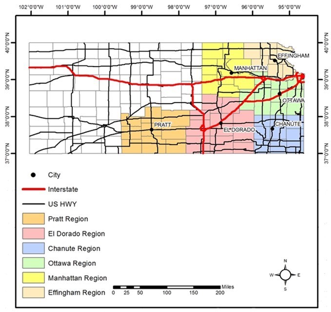
Fig. 1. The US FS FIA regions of interest

The Subregional Timber Supply (SRTS) model was used to estimate logging residue supply with recovery rates set to 30% (Abt et al. 2000; Abt 2008). The SRTS model uses USDA FS FIA data to project timber supply trends based on current conditions and the economic responses in timber markets (Abt and Cubbage 2000; Abt 2008). The internal inventory module in SRTS is based on the Georgia Regional Timber Supply (GRITS) model (Cubbage et al. 1990). The GRITS extrapolates forest inventories based on USDA FS FIA estimates of timberland area, timber inventory, timber growth rates, and timber removal. The GRITS classifies data into 10-year age class groups by broad species group (softwoods and hardwoods) and forest management type (planted pine, natural pine, oak-pine, upland hardwood, and lowland hardwood).

County-level forest quantity estimates were allocated to ZCTAs based on area proportionality and the land cover GIS imagery. If a ZCTA with all forestland accounts for 10% of a county, 10% of the county’s forest quantity was assigned to that ZCTA. The ArcGIS (Redlands, CA, USA) zonal histogram tool was used to determine the number of forest pixels in each county and ZCTA. The number of forest pixels in a given county, providing the forest quantity residing in each pixel, divided the county-level forest quantities. That ratio was then multiplied by the number of forest pixels in each ZCTA. When a ZCTA boundary crossed multiple counties, proportions for each county were summed. The ZCTAs were based on the 2010 census definition and obtained from the US Census Bureau (US Census Bureau 2010). The forest pixels were derived from the National Land Cover Database (2011). There were 4,486 supply ZCTAs (679 demand ZCTAs in KS) in the six-state study region with approximately 30% of them classified as excluded areas that are Federal lands, highly populated areas, and unsuitable ecoregions.

Forest Resource Costs

Resource cost data for woody cellulosic biomass was obtained from Timber Mart-South (2016). The average price data for Arkansas was used in the study, i.e., that is the only state close to KS that has periodic reported stumpage. There are currently no estimates for logging residue resource costs reported in the public domain. While some works did not include stumpage value of logging residues (Kerstetter and Lyons 2001; Gan and Smith 2006; Gan 2007), Wu et al. (2010) assumed the logging residue stumpage price to be 0.91 $ per green ton, Galik et al. (2009) gave a “rough approximation” of $1 per green ton. The value of 1$/green ton seemed underestimated, and therefore the logging residue stumpage price in this research was set to $1 per dry ton.

Harvesting Costs

Logging residue harvesting costs

The Fuel Reduction Cost Simulator (FRCS) as modified for the Billion Ton Study (Perlack et al. 2005; US Department of Energy 2011) by Dykstra (2008) was used to estimate the costs of harvesting logging residues (Stokes 1992; Fight et al. 2006). The revised FRCS (Dykstra 2008) was used to estimate logging residue costs for chipping tops and limbs at the landing, and in wood’s harvesting of sub-merchantable material.

Merchantable tree or roundwood harvesting costs

The Auburn Harvest Analyzer (AHA) (Auburn, AL, USA) was used to estimate harvesting costs for roundwood (Greene et al. 1987; Tufts et al. 1985; Tufts et al. 1988; Lanford and Stokes 1996). The AHA model was adapted for the six-state study region accounting for its ecoregions and forest stand types, and two available harvesting systems were assumed (e.g., feller-buncher/grapple skidder and chainsaw/cable skidder). The primary drivers for the model were the quadratic mean diameter, tons per acre removed, trees per acre removed, tract size, and average height of dominant trees obtained from the FIA merchantable tree estimates. The harvesting cost model generated roundwood production costs on a per dry ton basis for the two harvesting systems for all forest stand types. To evaluate the maximum available quantity of upland hardwood pulpwood in the region the authors assumed the use of a chainsaw/cable skidder and clearcut (where 100% of trees are removed) harvesting practices.

Transportation Costs

Transportation network

The shortest travel time routes between the demand and supply ZCTAs were estimated with Microsoft MapPoint 2011 (Redmond, WA, USA). The road networks in MapPoint are a combination of the Geographic Data Technology, Inc. (GDT) and Navteq (Chicago, IL, USA) data (Huang et al. 2012). The GDT data were used for rural areas and small to medium size cities, while the Navteq data were used for major metropolitan areas. The GDT data are based on “Tele Atlas Dynamap Streets,” which are address level geocoding. When an address level geocode is not available, the GDT data set uses cascading accuracy at the ZIP+4, ZIP+2, and ZIP code centroid to return the highest level of geocode for the address. The ZIP code boundary data are based on the Dynamap/5-Digit ZIP code Boundary data from Tele Atlas North America. The Navteq maps provide a highly accurate representation of the detailed road network, including up to 260 attributes, such as turn restrictions, physical barriers and gates, one-way streets, restricted access, and relative road heights.

Trucking costs

The transportation cost model estimated the fixed and variable trucking costs, based on the shortest travel time and distance from the MapPoint road network of a sourcing area, and the maximum annual mileage for tractor-trailers (the travel distance, which influences fixed costs, was allocated over the tractor-trailer’s estimated annual miles, which was 100,000 miles for the tractor and dry van and flatbed trailers; 80,000 miles for the long-log trailers). Single-driver day cabs were assumed with a maximum one-day legal round-trip time of 11 h. As supported in the research by Perez-Verdin (2009), fleet carriers contracted by a manufacturer were also assumed in this study. The choice of the trailer-type in the trucking cost model depended on the type of feedstock and was either dry-van storage for logging residues or full length for roundwood.

The trucking cost model was an adaptation of the truck transportation model by Berwick and Farooq (2003). The trucking variable costs were a function of travel time between the supply and demand ZCTAs, while the trucking fixed costs were a function of travel distance. The least-cost solutions for a set of supply ZCTAs to meet a specified demand quantity (i.e., 250,000 dry tons [226,750 metric tons] of logging residue) within a specified distance of 80 miles (128.7 km) were generally dependent on the shortest travel time between the supply and demand ZCTAs.

The trucking fixed costs included the equipment depreciation cost, average value of investment, interest, insurance, and taxes. Variable costs consisted of maintenance and repairs, diesel fuel and lubricants, and labor costs. The diesel fuel costs were obtained from the Energy Information Administration 2016 (Ferreira-Leitao et al. 2010) and are updated on monthly basis in the KS BioSAT model. Only ZCTAs able to supply at least one full truckload of biomass were considered for the analyses. The gross truck weight in the model was the 80,000-pound legal limit for KS (40 dry tons or 36.3 metric tons) (K.S.A. 8-1912).

Exclusion Criteria

The exclusion criteria were developed as a refinement of the available supply given legal, political, and social constraints for procuring sustainable woody biomass supply. For example, the production of commercial timberland is improbable in heavily populated areas (Wear et al. 1999); ZCTAs with a population density higher than 150 people per mi² (58 people per km²) were excluded from the analyses (Fig. 2). The ZCTAs within the US Environmental Protection Agency (EPA) Level III ecoregions (Fig. 3) that are not ecologically suitable for forest production (i.e., Nebraska Sand Hills, Northern Glaciated Plains, etc.) (US Environmental Protection Agency 2013) were excluded. Certain types of federal ownership were also excluded (i.e., Air Force Department of Defense (DOD), Bureau of Reclamation (BOR), National Grassland, Indian Reservations, etc.), as shown in Fig. 4.

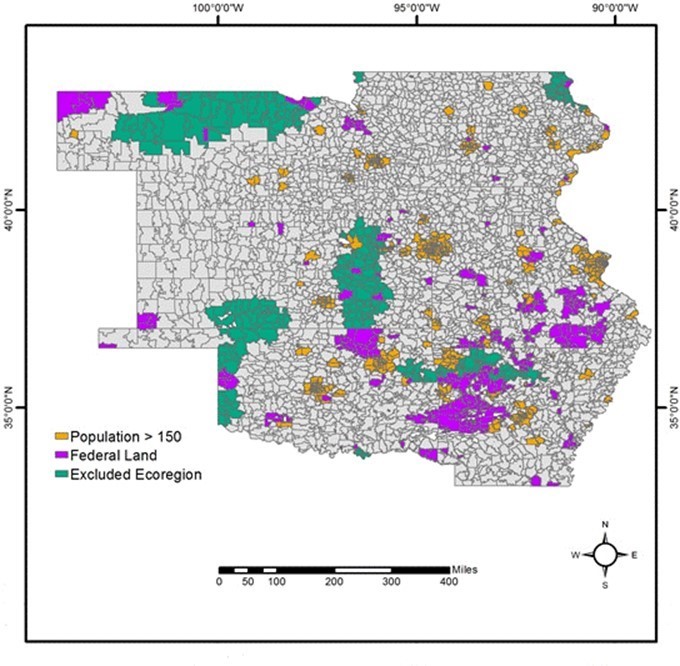
Fig. 2. Excluded zones due to population density, federal land, and EPA Level III ecoregions

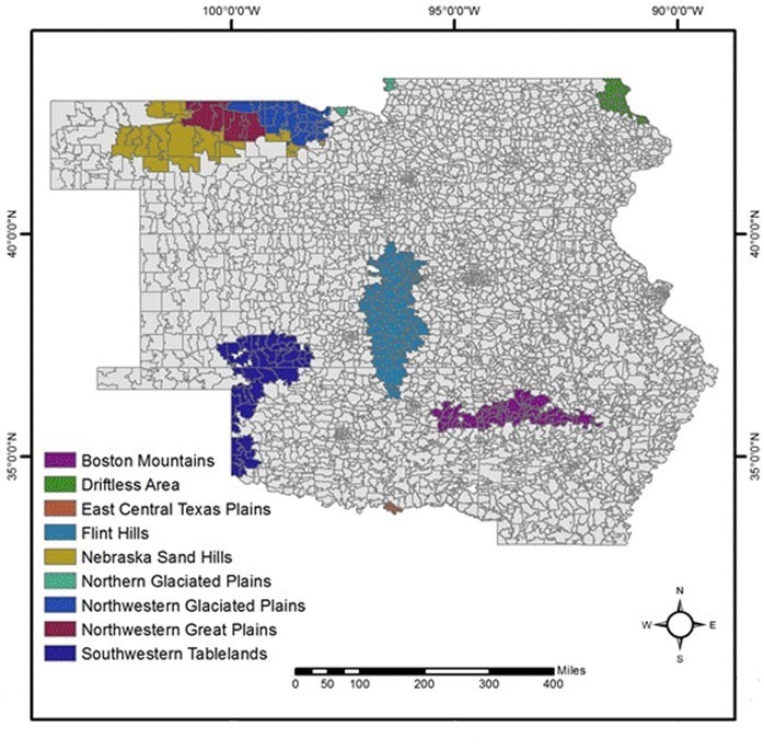
Fig. 3. Excluded US EPA Level III Ecoregions

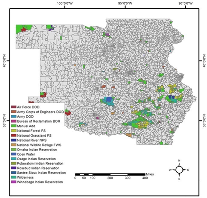
Fig. 4. Federal land excluded by type of federal ownership

RESULTS AND DISCUSSION

Logging Residues

The maximum quantity available in a sourcing area and the associated total cost, average total cost per dry ton (ATC), and median MC in dollars per dry ton were estimated for hardwood logging residues (at-landing and in-woods). Approximately 23 million dry tons (21 million metric tons) of hardwood logging residues were available in the six-state region, with only 0.9% located in KS (USDA 2015). The maximum annual quantity of hardwood logging residues available across all regions, within an 80-mile (128.7 km) one-way truck haul distance in KS, was a quarter of a million dry tons with the procurement areas predominately located in Missouri (Fig. 5).

The top ten ZCTAs (Figs. 5 and 6) were located in southeast Kansas for both of the hardwood logging residue types (at-landing and in-woods). The ATC per dry ton in the least-cost sourcing areas ranged from $22.86 to $24.72 per dry ton ($25.20 to $27.25 per metric ton) for at-landing, and from $146.88 to $147.36 per dry ton ($161.94 to $162.47 per metric ton) for in-woods logging residue. The median MC ranged from $23.41 to $26.92 per dry ton ($25.81 to $29.68 per metric ton) (Table 1, Fig. 7) for at-landing, and from $146.47 to $148.46 per dry ton ($161.49 to $163.68 per metric ton) for in-woods logging residue (Table 1, Fig. 7).

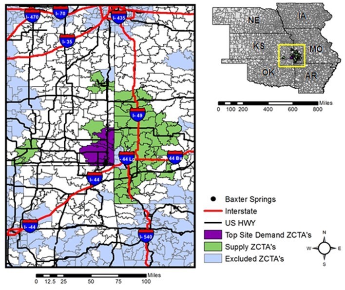
Fig. 5. Least-cost sourcing areas for at-landing hardwood logging residues in KS

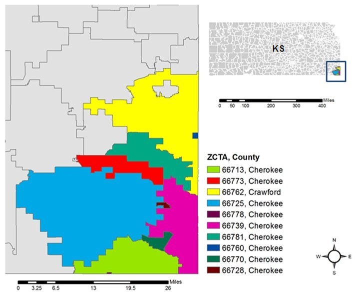
Fig. 6. Top ten demand ZCTAs for at-landing hardwood logging residues in KS

Table 1. Top Ten Locations in KS for At-Landing Hardwood Logging Residues, Based on Average Total Cost per Dry Ton

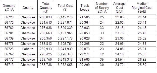
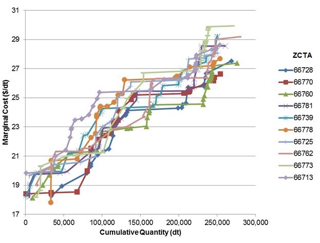
Fig. 7. Marginal cost curves for top ten locations for at-landing hardwood logging residues in KS

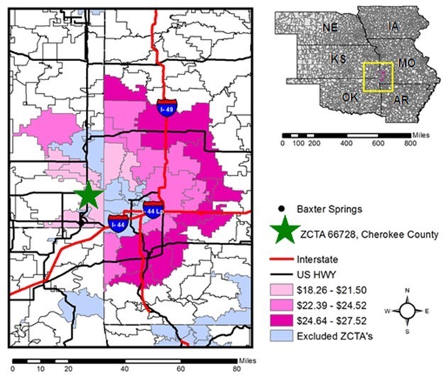
Fig. 8. Least-cost sourcing area for at-landing hardwood logging residues (ZCTA 66728, Cherokee County, KS)

Least-cost demand ZCTA for at-landing hardwood logging residues

The demand ZCTA 66728 (Cherokee County, KS) had the least ATC per dry ton of at-landing hardwood logging residues (Table 1). A quarter of a million dry tons of at-landing hardwood logging residues were available within an 80-mile (128.7 km) radius from ZCTA 66728 (Fig. 8). The MC ranged from $18.26 per dry ton to $27.52 per dry ton ($20.13 per metric ton to $ 30.41 per metric ton) (Fig. 9 and Table 2).

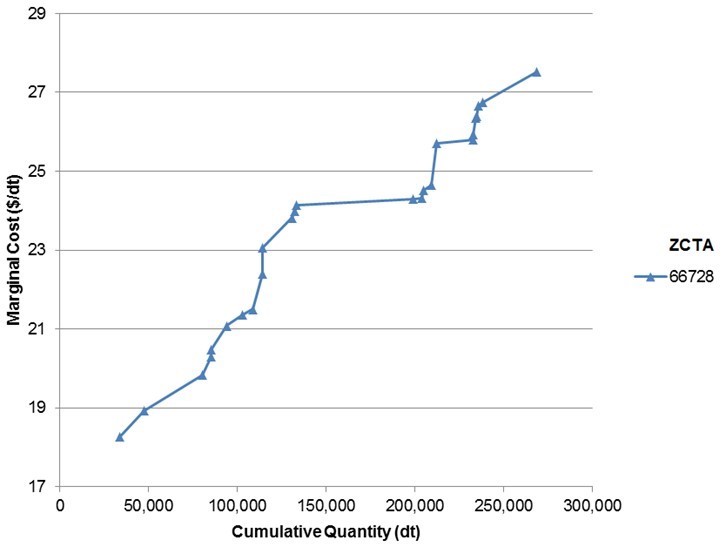
Fig. 9. Marginal cost curve for at-landing hardwood logging residues (ZCTA 66728, Cherokee County, KS)

Least-cost demand ZCTA for in-woods hardwood logging residues

The same top ten ZCTAs were selected for in-woods, as well as for the at-landing hardwood logging residues, because the analyses were based on the same resource data with the distinct difference in cost components. A quarter of a million dry tons of in-woods hardwood logging residues were available within an 80-mile (128.7 km) radius from ZCTA 66728 (Cherokee County, KS). The MC in the selected least-cost sourcing area ranged from $136.87 to $148.85 per dry ton ($150.90 to $164.11 per metric ton).

Upland Hardwood Pulpwood

The analyses of the six sub-regions of the state of Kansas for upland hardwood pulpwood net growth revealed that the Effingham, Ottawa, and Chanute in the more eastern regions of KS have a larger amount of woody biomass supply available within an 80-mile (128.7 km) one-way truck haul distance, relative to the other three regions (Table 3, Fig. 10).

Table 2. Supply ZCTAs for at-landing Hardwood Logging Residues in KS (Demand ZCTA 66728, Cherokee County)

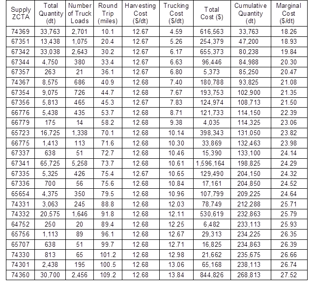
Table 3. Summary of Six US Forest Service FIA Sub-Regions in the State of Kansas

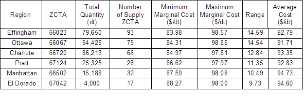
The Effingham region has the least MC per dry ton for upland hardwood pulpwood net growth, with procurement areas extending to Kansas, Missouri, and Nebraska. The ZCTA 66023 (Atchison County, KS) was the least-cost demand ZCTA in the Effingham region.

There are 93 supply ZCTAs within an 80-mile (128.7 km) radius from the ZCTA 66023 (Fig. 11) with an available cumulative annual quantity supply of 79,650 dry tons (72,242 dry metric tons) for upland hardwood pulpwood net growth. The MC for upland hardwood pulpwood net growth in the Effingham region ranged from $83.98 to $98.57 per dry ton ($92.59 to $108.68 per dry metric ton), while it ranged from $86.62 to $97.97 per dry ton ($95.50 to $108.02 per dry metric ton) in the Pratt region. It ranged from $84.31 to $98.85 per dry ton ($92.95 to $108.99 per dry metric ton) in the Ottawa region, and from $87.59 to $98.08 per dry ton ($96.57 to $108.14 per dry metric ton) in the Manhattan region.

The MC ranged from $88.27 to $98.00 per dry ton ($97.32 to $108.05 per dry metric ton) in the El Dorado region, and from $84.97 to $97.81 per dry ton ($93.68 to $107.84 per dry metric ton) in the Chanute region (Table 3, Fig. 12).

The cost estimates of this study were slightly higher in nominal dollars than those ($72.10 per dry ton [$79.49 per dry metric ton] with a maximum cost of $78.76 per dry ton [$86.84 per metric ton]) reported for Arkansas by Stokes (1992). However, this study had lower cost estimates by approximately 25%, when compared in real dollars to the study by Stokes (1992). This study also had a much more detailed transportation model than that of Stokes (1992).

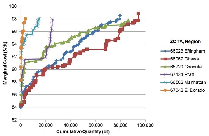
Fig. 10. The marginal cost curves for upland hardwood pulpwood net growth, analyses for six US Forest Service FIA sub-regions in the state of Kansas

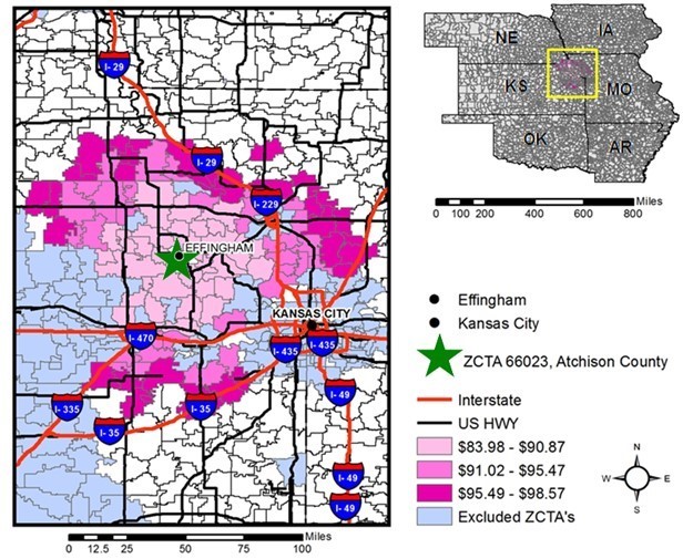
Fig. 11. The least-cost sourcing area for upland hardwood pulpwood net growth (ZCTA 66023, Atchison County, KS), relating to the Effingham region

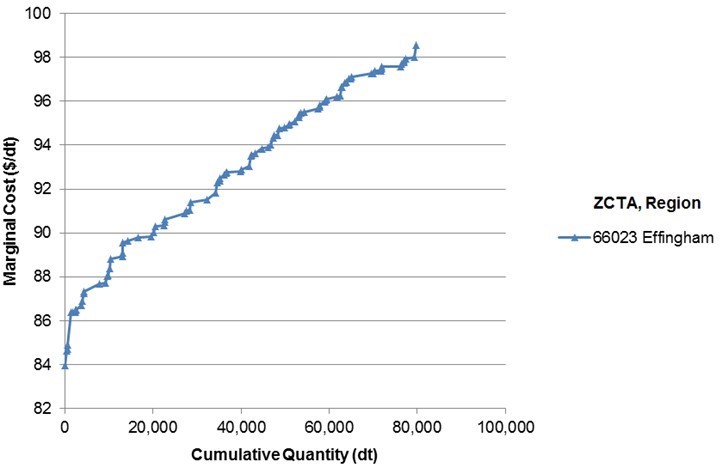
Fig. 12. Effingham Region. Marginal cost curve for upland hardwood pulpwood net growth (ZCTA 66023, Atchison County, KS)

CONCLUSIONS

This study improves the overall understanding of the economic costs of cellulosic feedstocks for potential manufacturers wishing to invest in the state of Kansas.
It provides decision-makers in the cellulosic feedstock-using industries with a better geospatial economic web-based tool that allows them to assess the economic comparative advantages of cellulosic supply from procurement zones within KS and from five surrounding states.
The KS BioSAT model may provide a useful template for other research conducted on the economic supply of woody biomass.
Least cost ZCTAs for at-landing and in-woods hardwood logging residue types were found in Southeastern Kansas. The average total costs in the areas were very similar with minimum of $22.86 per dry ton and maximum of $24.72 per dry ton for at-landing hardwood logging residue. The costs for in-woods logging residue were much higher, as was expected, and ranged from $146.88 to $147.36 per dry ton. Least cost ZCTA for upland hardwood pulpwood in the six KS sub-regions was found in Effingham region, Northeastern Kansas. Marginal costs in the region ranged from $83.98 to $98.57 per dry ton of upland hardwood pulpwood and were slightly higher in nominal dollars than those ($72.10 to $78.76 per dry ton) reported for Arkansas by Stokes (1992).

ACKNOWLEDGMENTS

Acknowledgments are extended to the staff from the US Forest Service (FS), Forest Inventory and Analysis (FIA) for providing the data and guidance. Special thanks go to Mr. Pat Miles of the US Forest Service. Kansas State University provided administrative support during the project. The funding for this project were on behalf of the Kansas Forest Service, United States Department of Agriculture (USDA) Forest Service, and McIntire-Stennis TENOOMS-107, which was administered by The University of Tennessee Agricultural Experiment Station.

REFERENCES CITED

Abt, R. C. (2008). “Sub-regional timber supply model- data, model, and projection updates,” in: Southern Forest Assessment Consortium IV, North Carolina State University, Raleigh, NC.

Abt, R. C., Cubbage, F. W., and Pacheco, G. (2000). “Southern forest resource assessment using the Subregional Timber Supply (SRTS) model,” Forest Prod. J. 50(4), 25-33.

Banks, D. I., Griffin, N. J., Shackleton, C. M., Shackleton, S. E., and Mavrandonis, J. M. (1996). “Wood supply and demand around two rural settlements in a semi-arid savanna, South Africa,” Biomass Bioenerg. 11(4), 319-331. DOI: 10.1016/0961-9534(96)00031-1

Berwick, M., and Farooq, M. (2003). “Trucking cost model for transportation managers,” Upper Great Plains Transportation Institute, North Dakota State University, Fargo, ND.

Biomass Research and Development Board (2010). “Increasing feedstock production for biofuels economic drivers, environmental implications, and the role of research,” Biomass Research and Development Initiative, (http://www.biomassboard.gov/pdfs/8_Increasing_Biofuels_Feedstock_Production.pdf).

Brown, S. L., and Schroeder, P. E. (1999). “Spatial patterns of aboveground production and mortality of woody biomass for eastern US forests,” Ecol. Appl. 9(3), 968-980. DOI: 10.2307/2641343

Champagne, P. (2007). “Feasibility of producing bio-ethanol from waste residues: A Canadian perspective: Feasibility of producing bio-ethanol from waste residues in Canada,” Resour. Conserve. Recy. 50(3), 211-230. DOI: 10.1016/j.resconrec.2006.09.003

Cubbage, F. W., Hogg, D. W., Harris, T. G., and Alig, R. J. (1990). “Inventory projection with the Georgia Regional Timber Supply (GRITS) model,” South. J. Appl. For. 14(3), 137-142.

Dasappa, S. (2011). “Potential of biomass energy for electricity generation in sub-Saharan Africa,” Energ. Sust. Dev. 15(3), 203-213. DOI: 10.1016/j.esd.2011.07.006

De Wit, M., and Faaij, A. (2010). “European biomass resource potential and costs,” Biomass Bioenerg. 34(2), 188-202. DOI: 10.1016/j.biombioe.2009.07.011

DiPardo, J. (2000). “Outlook for biomass ethanol production and demand,” Energy Information Administration, (http://indigowatergroup.com/Files/CSM%202012/09%20-%20Energy%20Conservation/Ethanol%20Production%20and%20Demand.pdf).

Downing, M., and Graham, R. L. (1996). “The potential supply and cost of biomass from energy crops in the Tennessee valley authority region,” Biomass Bioenerg. 11(4), 283-303. DOI: 10.1016/0961-9534(96)00004-9

Dykstra, D. P. (2008). Subject: Estimating Biomass Collection Costs for the “Billion-Ton Study” update. Memo: Estimating Forest Biomass Collection Costs for the Billion-Ton Study Update (BTS2), US Department of Agriculture, Forest Service.

Energy Information Administration (2016). “Weekly retail on-highway diesel prices,” (http://tonto.eia.doe.gov/oog/info/wohdp/diesel.asp), accessed 14 March 2016.

Camas Creek Enterprises, Inc. (2009). “Kansas state-wide woody biomass supply and utilization assessment,” Kansas Forest Service, Manhattan, KS.

Ferreira-Leitao, V., Gottschalk, L. M. F., Ferrara, M. A., Nepomuceno, A. L., Molinari, H. B. C., and Bon, E. P. (2010). “Biomass residues in Brazil: Availability and potential uses,” Waste Biomass Valor. 1(1), 65-76. DOI: 10.1007/s12649-010-9008-8

Fight, R. D., Hartsough, B. R., and Noordijk, P. (2006). Users Guide for FRCS: Fuel Reduction Cost Simulator Software (PNW-GTR- 668), U.S. Department of Agriculture Pacific Northwest Research Station, Portland, OR.

Galik, C. S., Abt, R. C., and Wu, Y. (2009). “Forest biomass supply in the southeastern United States- Implications for industrial roundwood and bioenergy production,” J. Forest 107(2), 69-77.

Gan, J. (2007). “Supply of biomass, bioenergy, and carbon mitigation: Method and application,” Energy Policy 35(12), 6003-6009. DOI:10.1016/j.enpol.2007.08.014

Gan, J., and Smith, C. T. (2006). “Availability of logging residues and potential for electricity production and carbon displacement in the USA,” Biomass Bioenerg. 30(12), 1011-1020. DOI:10.1016/j.biombioe.2005.12.013

Greene, W. D., Lanford, B. L., and Hool, J. N. (1987). “Potential product volumes from 2^nd thinnings of southern pine plantations,” Forest Prod. J. 37(5), 8-12.

Houghton, R. A., Lawrence, K. T., Hackler, J. L, and Brown, S. (2001). “The spatial distribution of forest biomass in the Brazilian Amazon: A comparison of estimates,” Glob. Change Biol. 7(7), 731-746. DOI: 10.1111/j.1365-2486.2001.00426.x

Huang, X., Perdue, J. H., and Young, T. M. (2012). “A spatial index for identifying opportunity zones for woody cellulosic conversion facilities,” Int. J. Forest Res. 2012, 106474. DOI: 10.1155/2012/106474

Joshi, P., Sharma, N., and Manab Sarma, P. (2016). “Assessment of biomass potential and current status of bio-fuels and bioenergy production in India,” Current Biochem. Eng. 3(1), 4-15. DOI: 10.2174/2212711902999150923155545

Kansas Forest Service. (2015). A Road Map for Kansas Forests, Woodlands, and Windbreaks, Kansas Forest Service, Manhattan, KS.

Kansas State Law (2016). “Vehicle weight limits K. S. A. 8-1901-8-1912,” Topeka Municipal Code, Topeka, KS.

Kerstetter, J. D., and Lyons J. K. (2001). “Logging and agricultural residue supply curves for the Pacific Northwest,” Washington State University Energy Program. DOI: 10.2172/900299

Koopmans, A. (2005). “Biomass energy demand and supply for South and South-East Asia- Assessing the resource base,” Biomass Bioenerg. 28(2), 133-150. DOI: 10.1016/j.biombioe.2004.08.004

Lanford, B. L., and Stokes, B. J. (1996). “Comparison of two thinning systems. Part 2. Productivity and costs,” Forest Prod. J. 46(11-12), 47-53.

Langholtz, M. H., Stokes, B. J., and Eaton, L. M. (2016). 2016 Billion-Ton Report: Advancing Domestic Resources for a Thriving Bioeconomy, Volume 1: Economic Availability of Feedstocks (ORNL/TM-2016/160), Oak Ridge National Laboratory, Oak Ridge, TN.

Marrison, C. I., and Larson, E. D. (1996). “A preliminary analysis of the biomass energy production potential in Africa in 2025 considering projected land needs for food production,” Biomass Bioenerg. 10(5), 337-351. DOI: 10.1016/0961-9534(95)00122-0

Munsell, J. F., and Fox, T. R. (2010). “An analysis of the feasibility for increasing woody biomass production from pine plantations in the southern United States,” Biomass Bioenerg. 34(12), 1631-1642. DOI: 10.1016/j.biombioe.2010.05.009

Nakada, S., Saygin, D., and Gielen, D. (2014). “Global BioEnergy Supply and Demand projection: A working paper for REmap 2030,” International Renewable Energy Agency (IRENA), 1-88.

National Land Cover Database (2011). “National land cover database 2011,” (http://www.mrlc.gov/nlcd11_data.php), accessed 7 October 2014.

Oak Ridge National Laboratory, Biomass Energy Data Book, (http://cta.ornl.gov/bedb/appendix_a.shtml), accessed 10 February 2015.

Perdue, J. H., Young, T. M., and Rials, T. G. (2011). The Biomass Site Assessment Model- BioSAT, U.S. Forest Service Southern Research Station, Knoxville, TN.

Perlack, R. D., and Stokes, B. J. (2011). US Billion-ton update, Biomass Supply for a Bioenergy and Bioproducts Industry (ORNL/TM-2011/224), Oak Ridge National Laboratory, Oak Ridge, TN.

Perlack, R. D., Wright, L. L., Turhollow, A. F., Graham, R. L., Stokes, B. J., and Erbach, D. C. (2005). Biomass as Feedstock for a Bioenergy and Bioproducts Industry: The Technical Feasibility of a Billion-Ton Annual Supply (DOE/GO-102995-2135/ORNL TM-2005/66), OAK Ridge National Laboratory, Oak Ridge, TN.

Perez-Verdin, G., Grebner, D. L., Sun, C., Munn, I. A., Schultz, E. B., and Matney, T. G. (2009). “Woody biomass availability for bioethanol conversion in Mississippi,” Biomass Bioenerg. 33(3), 492-503. DOI: 10.1016/j.biombioe.2008.08.021

Rytter, L., Andreassen, K., Bergh, J., Ekö, P. M., Grönholm, T., Kilpeläinen, A., Lazdina, D., Muiste, P., and Nord-Larsen, T. (2015). “Availability of biomass for energy purposes in Nordic and Baltic countries: Land areas and biomass amounts,” Balt. For. 21(2), 375-390.

Sasaki, N., Knorr, W., Foster, D. R., Etoh, H., Ninomiya, H., Chay, S., Kim, S., and Sun, S. (2009). “Woody biomass bioenergy potentials in Southeast Asia between 1990 and 2020,” Appl. Energy 86(S1), S140-S150. DOI: 10.1016/j.apenergy.2009.04.015

Skog, K. E., and Barbour R. J. (2006). “Estimating woody biomass supply from thinning treatments to reduce fire hazard in the US West,” in: Fuels Management- How to Measure Success Conference Proceedings, Fort Collins, CO, pp. 657-672.

Stokes, B. J. (1992). “Harvesting small trees and forest residues,” Biomass Bioenerg. 2(1), 131-147. DOI: 10.1016/0961-9534(92)90095-8

Timber Mart-South (2016). “Quarterly report of the market prices for timber products of the Southeast. 4^th Quarter 2015,” J. South. Timb. Prices 40(4).

Tufts, R. A., Lanford, B. L., Greene, W. D., and Burrows, J. O. (1985). “Auburn harvesting analyzer,” The Compiler 3(2), 14-15.

Tufts, R. A., Stokes, B. J., and Lanford, B. L. (1988). “Productivity of grapple skidders in southern pine,” Forest Prod. J. 38(10), 24-30.

Ugarte, D. L. T., English, B. C., and Jensen, K. (2007). “Sixty billion gallons by 2030: Economic and agricultural impacts of ethanol and biodiesel expansion,” Am. J. Agr. Econ. 89(5), 1290-1295. DOI: 10.1111/j.1467-8276.2007.01099.x

US Census Bureau (2010). “ZIP code tabulation area (ZCTA) for Census 2010,” (https://www.census.gov/en.html), accessed 26 August 2014.

US Department of Agriculture Forest Service (2015). “Forest and inventory national database 3.0,” (http://www.fia.fs.fed.us/tools-data/), accessed 5 August 2015.

US Department of Energy (2016). “Alternative fuels data center,” (http://www.afdc.energy.gov/fuels/ethanol_feedstocks.html), accessed 28 March 2016.

US Environmental Protection Agency. (2013). “US Level III and IV Ecoregions,” (https://www.epa.gov/eco-research/level-iii-and-iv-ecoregions-continental-united-states), accessed 10 February 2015. []

Verkerk, P. J., Anttila, P., Eggers, J., Lindner, M., and Asikainen, A. (2011). “The realisable potential supply of woody biomass from forests in the European Union,” Forest Ecol. Manag. 261(11), 2007-2015. DOI: 10.1016/j.foreco.2011.02.027

Walsh, M. E. (2008). “US cellulosic biomass feedstock supplies and distribution,” M & E Biomass 2008, 1-47.

Wear, D. N., Liu, R., Foreman, J. M., and Sheffield, R. M. (1999). “The effects of population growth on timber management and inventories in Virginia,” Forest Ecol. Manag. 118(1), 107-115. DOI: 10.1016/S0378-1127(98)00491-5

Welfle, A., Gilbert, P., and Thornley, P. (2014). “Increasing biomass resource availability through supply chain analysis,” Biomass Bioenerg. 70, 249-266. DOI: 10.1016/j.biombioe.2014.08.001

White, E. M. (2010). Woody Biomass for Bioenergy and Biofuels in the United States: A Briefing Paper (PNW-GTR-825), U.S. Department of Agriculture Pacific Northwest Research Station, Portland, OR.

Wu, J., Sperow, M., and Wang, J. (2010). “Economic feasibility of a woody biomass-based ethanol plant in central Appalachia,” J. Agr. Resour. Econ. 522-544.

Yoshioka, T., Hirata, S., Matsumura, Y., and Sakanishi, K. (2005). “Woody biomass resources and conversion in Japan: The current situation and projections to 2010 and 2050,” Biomass Bioenerg. 29(5), 336-346. DOI: 10.1016/j.biombioe.2004.06.016

Young, T. M., and Ostermeier, D. M. (1989). IFCHIPSS-The Industrial Fuel Chip Supply Simulation Model (Final Report), Southeastern Regional Biomass Energy Program, Tennessee Valley Authority, 141 p.

Young, T. M., Ostermeier, D. M., Thomas, J. D., and Brooks, R. T. (1991). “The economic availability of woody biomass for the Southeastern United States,” Bioresource Technol. 37(1), 7-15. DOI: 10.1016/0960-8524(91)90106-T

Zalesny, R. S., Stanturf, J. A., Gardiner, E. S., Perdue, J. H., Young, T. M., Coyle, D. R., Headlee, W. L., Banuelos, G. S., and Hass, A. (2016). “Ecosystem services of woody crop production systems,” BioEnergy Research 9(2), 465-491. DOI: 10.1007/s12155-016-9737-z

Zambelli, P., Lora, C., Spinelli, R., Tattoni, C., Vitti, A., Zatelli, P., and Ciolli, M. (2012). “A GIS decision support system for regional forest management to assess biomass availability for renewable energy production,” Environ. Modell. Softw. 38(12), 203-213. DOI: 10.1016/j.envsoft.2012.05.016

Article submitted: October 17, 2016; Peer review completed: November 26, 2016; Revised version received and accepted: December 2, 2016; Published: December 9, 2016.

DOI: 10.15376/biores.12.1.960-980

BioResources

Geospatial economics of the woody biomass supply in Kansas – A case study

Abstract

Full Article