
Abstract
The equilibrium moisture content and specific gravity of Uludag fir (Abies bornmüelleriana Mattf.) and hornbeam (Carpinus betulus L.) woods were investigated following heat treatment at different temperatures and times. Two prediction models were established based on the Aquila optimization algorithm back-propagation neural network model. To demonstrate the effectiveness and accuracy of the proposed model, it was compared with a tent sparrow search algorithm-back-propagation network model, a back-propagation network model, and an artificial neural network. The results showed that the Aquila optimization algorithm back-propagation model reduced the root mean square error value of the original back-propagation model by 87% and 97%, respectively, and the decision coefficients (R2) of the equilibrium moisture content and specific gravity were 0.99 and 0.98; as such, the model optimization effect was obvious. Therefore, this paper provides an effective method for the optimization of the process parameters (such as heat treatment time, temperature, and air pressure) in wood heat treatment and related fields.
Download PDF
Full Article
Prediction of the Equilibrium Moisture Content and Specific Gravity of Thermally Modified Wood via an Aquila Optimization Algorithm Back-propagation Neural Network Model
Yao Chen, Wei Wang,* and Ning Li
The equilibrium moisture content and specific gravity of Uludag fir (Abies bornmüelleriana Mattf.) and hornbeam (Carpinus betulus L.) woods were investigated following heat treatment at different temperatures and times. Two prediction models were established based on the Aquila optimization algorithm back-propagation neural network model. To demonstrate the effectiveness and accuracy of the proposed model, it was compared with a tent sparrow search algorithm-back-propagation network model, a back-propagation network model, and an artificial neural network. The results showed that the Aquila optimization algorithm back-propagation model reduced the root mean square error value of the original back-propagation model by 87% and 97%, respectively, and the decision coefficients (R2) of the equilibrium moisture content and specific gravity were 0.99 and 0.98; as such, the model optimization effect was obvious. Therefore, this paper provides an effective method for the optimization of the process parameters (such as heat treatment time, temperature, and air pressure) in wood heat treatment and related fields.
DOI: 10.15376/biores.17.3.4816-4836
Keywords: BP neural network model; Aquila optimization; Heat treatment; Equilibrium moisture content; Specific gravity
Contact information: College of Engineering and Technology, Northeast Forestry University, Harbin 150040 China; *Corresponding author: vickywong@nefu.edu.cn
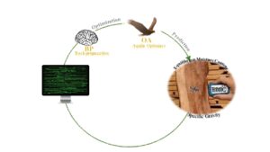
GRAPHICAL ABSTRACT
INTRODUCTION
Fir and hornbeam are important tree species in the timber industry. Fir wood can be used for indoor flooring and furniture, as well as outdoor building materials and shipbuilding. However, fir has problems such as low strength and poor dimensional stability, and its equilibrium moisture content is largely affected by the heat treatment temperature. Hornbeam wood is tough and can be used to make farm implements, furniture, daily gadgets, etc. However, hornbeam wood has a fine grain and will experience significant mass loss after heat treatment, resulting in a decrease in density (Gunduz et al. 2009). Therefore, it is of great significance for the wood processing industry to study the properties of Uludag fir and hornbeam after heat treatment.
The treatment process does not introduce chemicals, so heat treatment is generally regarded as an environmentally friendly modification method that has received extensive attention (Esteves and Pereira 2009). Stamm and Hansen (2002) used various gases to heat wood to reduce its shrinkage and swelling. Cronin et al. (2003) gave expressions for predicting the mean and standard deviation of the sheet moisture content over time. At the same time, a comparison with the Monte Carlo model was carried out, and a dual set point planning model was proposed.
Fortin et al. (2004) proposed a two-dimensional wood drying model based on the concept of water potential to simulate convective batch drying of wood at conventional temperatures. The model can be well combined with an intelligent adaptive kiln controller for an online optimized drying schedule. Oumarou et al. (2015) proposed the 3D modeling of high-temperature heat-treated wood. Neural networks are the primary branch of intelligent control technology research in recent years. Because of its parallel processing, self-adaptation, self-learning, and good fault tolerance, it has been widely used in the actual drying industry. Numerous studies on the application of artificial neural networks to the properties of wood after heat treatment can be found in the literature. Some of these studies are summarized as follows:
Farkas et al. (2000) established a neural network grain drying model. Nasir et al. (2019), using the stress wave method, established an adaptive neuro-fuzzy inference system (ANFIS) and a neural network (NN) model to predict the properties of thermally modified wood. Watanabe et al. (2013), based on the artificial neural network model, evaluated the final moisture content of fir wood and compared the data with the principal component regression (PCR) model, and concluded that the ANN model was more accurate.
Tiryaki and Aydin (2014) used artificial neural networks to predict the compressive strength of heat-treated wood along the grain and compared the results with the multiple linear regression model; the results showed that artificial neural network yielded a better prediction effect. Chai et al. (2018), based on the BP (back propagation) neural network algorithm, predicted the change in the wood moisture content (MC) during high-frequency vacuum drying. Compared with the experimental measurement results, the predicted value conformed to the change law and size of the experimental value.
However, BP neural network has the disadvantages of easily falling into local minimum and slow training speed. Therefore, it is difficult for a single BP algorithm to meet the requirements of prediction accuracy. Many scholars choose to use metaheuristic methods to optimize the parameters of BP to improve the prediction accuracy. Metaheuristic methods simulate the behavior of animals in nature. Commonly used metaheuristic algorithms include the genetic algorithm, ant colony algorithm, simulated annealing method, etc. In this paper, a new algorithm is proposed for the prediction of the equilibrium moisture content (EMC) and specific gravity (SG) in the drying process. Specifically, Aquila optimization (AO) is used to optimize the weights and thresholds of the BP neural network. Through the comparison of multiple indicators, the superiority of the method was confirmed, and the prediction accuracy of the equilibrium moisture content and specific gravity of the wood during the drying process was improved. As such, this model has certain academic importance and application value in the research field of wood drying technology.
In summary, there are many studies on heat-treated wood, but there is still a lot of room for improvement in prediction accuracy and training speed. This paper proposes an Aquila optimization algorithm back-propagation neural network model (AO-BP) algorithm to predict the equilibrium moisture content and specific gravity of wood and compares it with multiple models to demonstrate the validity and accuracy of the AO-BP model.
EXPERIMENTAL
Materials
To ensure the subsequent more accurate comparison of the results of the algorithms, this paper used the same data as Ozsahin and Murat (2018). The authors used data for the Uludag fir (Abies bornmüelleriana Mattf.) and hornbeam (Carpinus betulus L.) wood species. The samples were sourced from a local sawmill in Turkey and were taken from the sapwood area of a single log of each type of wood, the dimensions of which were 20 mm × 20 mm × 30 mm (L × R × T). Before heat treatment, all samples were conditioned at a temperature of 20 °C ± 1 °C and a relative humidity of 65% ± 1% until they reached the equilibrium moisture content. The test material was heat-treated under normal pressure, and the thermal modification process parameters were the temperature, time, and relative humidity. The test samples were heat-treated in a fully controlled oven with a sensitivity of ± 1 °C, three levels of thermal modification temperatures (170, 190, and 210 °C), and three levels of heat treatment time (4, 8, and 12 h). Different temperatures and treatment times can be combined into 9 combinations, of which 10 samples and 10 control groups (200 samples each for the Uludag fir and hornbeam species) were taken for the determination of the specific gravity and equilibrium moisture content values. In addition, ISO standard 13061-1 (2014), ISO standard 13061-2 (2014), and ISO standard 3129 (2012) were used to determine specific gravity and equilibrium moisture content of heat-treated samples at a temperature of 20 °C and a relative humidity of 35%, 50%, 65%, 80%, and 90%.
Methods
Back-propagation neural network model
A back-propagation (BP) neural network is a multi-layer architecture with the input layer, output layer, and hidden layer. Figure 1 shows the structure of a BP neural network. The BP model contains two propagation processes, forward and reverse. In the forward propagation process, the samples are processed from the input layer through the hidden layer neurons, and the output of each layer of neurons only affects the state of the next layer of neurons until the output. If there is a deviation between the output of the network and the expected output, back propagation is entered. During back propagation, the error signal is transmitted back from the original forward propagation path, and the weight coefficients of the neurons in each layer are corrected according to the negative gradient direction of the error function, and finally the error tends to be minimized.

Fig. 1. BP Network Structure
This work used the machine learning toolbox that comes with MATLAB (2018a) to create a BP network. The model used the wood species, temperature, relative humidity, and exposure period as the input layer data, and then used the EMC and SG as the output layer data, respectively. The data (90 samples) were divided into two groups, of which 60 samples were used as the training sets and 30 samples were used as the test sets.
To determine the optimal network architecture and parameters, a trial-and-error approach was employed. Several different BP network structures, parameters, and datasets were tested thousands of times using the developed software until the difference (error) between the measured and predicted values reached an acceptable level. After repeated trial and error, the number of hidden layer nodes of the BP network model was finally determined to be 7 and 16, respectively, and the mean square error of the model was the smallest at this time.
The sample data and the time axis must strictly correspond, and because the sample data has the problem of non-uniform dimensions, it is necessary to normalize the sample data to achieve the best generalization potential and performance of the AO-BP model. The normalization formula is shown in Eq. 1,
 (1)
(1)
where Xnorm is the normalized data, X is the original data, and Xmax and Xmin are the maximum and minimum values of the original data set, respectively.
Generally speaking, all nodes in the hidden layer use the Sigmoid transfer function, and in the output layer, all nodes use the linear transfer function Pureline. The Sigmoid function is shown in Eq. 2,
 (2)
(2)
where σ(x) is the neuron output value and x is the neuron input value.
In this paper, the trainlm() training function with the fastest convergence speed was used to establish a BP neural network simulation prediction model, with a learning rate set to 0.01.
Aquila optimizer model
The Aquila optimizer (AO) is a swarm-based meta-heuristic optimization method based on the natural behavior of an Aquila when catching prey (Abualigah et al. 2021). When Aquila hunts prey, there are four different predation behaviors for different prey, and these four behaviors correspond to four optimization processes, i.e., extended exploration, narrow exploration, extended exploitation, and narrowed exploitation in the AO algorithm.
The powerful global search ability of the AO can effectively optimize the initial weight and threshold of the BP network, avoiding the shortcomings of the traditional BP network, i.e., a slow convergence and easily falling into the local minimum. The algorithm flow of the AO-BP model is shown in Fig. 2.
Firstly, the population is initialize using Eq. 3,
 (3)
(3)
where r1 is a random value in [0, 1], UBj and LBj are the upper and lower bounds at dimension j, respectively, and dim is the dimension of the problem.

Fig. 2. The AO-BP algorithm flow chart
After the population is initialized, the AO algorithm is divided into two stages, i.e., exploration and exploitation. When t is less than or equal to 2/3*T, it is in the exploration stage. The specific optimization process of the AO algorithm is as follows:
1) Expanded exploration: Vertically pitch and fly high to select the hunting area.
An aquila conducts extensive exploration at high altitudes, identifies the area where the prey is located, and after determining the area where the prey is located, selects the best hunting location by bending down vertically. The equation is expressed as shown in Eq. 4,
 (4)
(4)
where X1(t+1) is the next solution after t iterations generated by the first search method X1, Xb(t) is the currently updated optimal solution, t and T represent the current number of iteration and the maximum number of iterations, respectively, and Xm(t) is the current solution after the average value of the t iterations, which was calculated using Eq. 5,
 (5)
(5)
where N is the population size.
2) Narrowed exploration: Contour flight and short-range attack.
After finding the area where the prey is located at high altitude, it hovers at a lower altitude above the prey, preparing for a short-range attack. At this stage, the current individual is updated using the levy flight distribution function, as shown in Eq. 6,
 (6)
(6)
where X2(t+1) represents the solution for the next iteration of t, XR(t) is the random solution for the ith iteration, x and y represents the shape of the downward spiral in the search for prey, as calculated by Eq. 7
 (7)
(7)
where r is calculated by Eq. 8,
 (8)
(8)
where r1 is a random value in [1-20], D1 is an integer, U equals 0.00565, ω equals 0.005, and Levy(D) is the levy flight function, which is obtained according to Eq. 9,
 (9)
(9)
where s is 0.001, u and υ are a random number in [0, 1], and σ is calculated by Eq. 10,
 (10)
(10)
where β is a constant value with a fixed bit of 1.5.
3) Extended exploitation: Low-altitude flight and slow descent attack.
After determining the approximate location of the prey, the Aquila prepares for vertical pre-attack, preying on the prey through a slow descent in low-flying flight. This behavior can be expressed by Eq. 11,
 (11)
(11)
where α and δ are the adjustment parameters fixed to a small value (0.1), and UB and LB are the upper and lower bounds, respectively.
4) Narrowed exploitation: Run on foot and catch prey.
When Aquila approaches the prey, it observes the escape trajectory of the prey and selects random movements to catch the prey on land by running and raiding, and is written as shown in Eq. 12 through Eq. 15,
 (12)
(12)
 (13)
(13)
 (14)
(14)
 (15)
(15)
where QF is the quality function value used for the balance search step, QF(t) is the the value of QF after t iterations, G1 represents the various motions generated in the process of finding the optimal solution, calculated by Eq. 14, and G2 is the flight slope of the AO as it follows its prey, described as a random value decreasing from 2 to 0.
RESULTS AND DISCUSSION
Model Evaluation Criteria
Statistical errors are often used to evaluate the predictive performance of a model. Commonly used regression evaluation indicators are the mean absolute (MAE), mean squared error (MSE), root mean squared error (RMSE), and mean absolute percentage error (MAPE). The RMSE and MSE are essentially the same, so only the RMSE was used in this article. This was because the MSE unit magnitude and error magnitude are different, and the RMSE belongs to the same level as the data, so the RMSE can better describe the data. In general, this paper selected the MAE, RMSE, and MAPE as the evaluation indicators of the model, and the calculation formulas are shown in Eq. 16 through Eq. 18, respectively,
 (16)
(16)
 (17)
(17)
 (18)
(18)
where Ai and Fi represent the actual value and the predicted value, respectively.
Model Performance Comparison Analysis
In this paper, the AO-BP algorithm was compared the BP, tent sparrow search algorithm-back-propagation (TSSA-BP), and ANN models. Among them, TSSA refers to using the Tent chaotic map to add a random sequence to improve the accuracy of the sparrow search algorithm (SSA) (Bing and Weisun 1997). In order to reduce disputes, this paper took the mean of 5 runs of the AO-BP model as the final results (Table 1).
Table 1. Aquila Optimization Back-propagation Model Running Results

The evaluation results of each model are listed in Table 2 (Appendix Tables A1 through A4 show the predicted values and errors for the training data and test data for each model). In particular, the prediction data of the ANN was taken from the research results of Ozsahin and Murat (2018). Compared with the unoptimized BP neural network, the AO-BP reduced the MAPE values of the training data of the EMC and SG models by 86% and 96%, respectively, and the RMSE by 87% and 97%, respectively. In addition, the MAE values were reduced by 86% and 97%, respectively. Furthermore, compared with the TSSA-BP and ANN models, the prediction results of the AO-BP model were closer to the actual value. This shows that the AO-BP model optimization effect was obvious. In addition, the RMSE when the AO-BP model predicts the SG was slightly higher than the RMSE of the ANN model, which may be due to the existence of jumping data, which leads to some discrete values in the prediction results. However, the MAPE and MAE of the AO-BP model were far lower than the prediction results of the ANN model, and the prediction effect of the AO-BP model was generally better.
Table 2. Model Evaluation Results


Fig. 3. Comparison graph of the training set for the (a) EMC and (b) SG
It can be seen from Figs. 3 and 4 that the actual and predicted values of the EMC and SG are very similar. This shows that the predicted value can better reflect the true value. The maximum number of iterations of the model was set to 1000 times. Taking the EMC as an example, the ANN, TSSA-BP, and AO-BP models were iterated 60, 23, and 6 times, respectively, which indicated that the AO-BP optimization model has a greater advantage in terms of the convergence speed when predicting the EMC.

Fig. 4. Comparison graph of the testing set for the (a) EMC and (b) SG
Linear Regression Analysis
This paper used linear regression to analyze the fitting effect of the model. The fitting effect is shown in Figs. 5a and 5b. The R-values of the EMC and SG in all data sets were greater than 0.99, and the target value and the output result were basically on the same straight line. This shows that there was a significant correlation between the measured and predicted values for all the data. In previous studies, Watanabe et al. (2013) using ANN to predict the MC of Sugi Lumber, the correlation coefficients of the training set and test sets were 0.91 and 0.8, respectively. Chai et al. (2018) using BP neural networks to predict MC, the R2 obtained was 0.974, which indicates that the model they proposed was able to explain more than 97% of the experimental value. In this paper, the R2 of EMC and SG, which were run five times, were 0.99 and 0.98, respectively. The results of these five operations were 0.99, 0.98, 0.99, 0.98, 0.99 and 0.98, 0.97, 0.99, 0.99, 0.97.

Fig. 5. Regression models for the (a) EMC and (b) SG
Phenomenon Analysis
Considering the problem of space, this paper only took the EMC of Uludag fir at a temperature of 210 °C and the SG at a relative humidity of 35% as examples. The data in Figs. 6 and 7 were derived from model predictions, and a comparison of these data and measurements is shown in the appendix. It can be seen from Figs. 6 and 7 that the changing trends of the EMC and SG of the heat-treated samples were consistent with those reported in by Gunduz et al. (2008). This again illustrates the effectiveness of the AO-BP model.
Both the equilibrium moisture content and specific gravity of the wood after heat treatment were lower than the EMC and SG of the control wood, and similar results were also reported in the literature (Kamdem et al. 2002; Korkut et al. 2008; Liu et al. 2014; Kocaefe et al. 2015). The reduction of the EMC is primarily caused by the reduction of hydroxyl number during the heat treatment of the wood. On one hand, the non-crystalline area of the celluloses and hemicelluloses are degraded, while on the other hand, cross-linking between the lignins occurs. Under the combined action of various factors, the EMC of wood after heat treatment is reduced (Tjeerdsma and Militz 2005; Boonstra and Tjeerdsma 2006).

Fig. 6. Effect of heat treatment at 210 °C on the equilibrium moisture content of Uludag fir
The specific gravity is the ratio of the wood density to the water density at a specific temperature, and the decrease in the specific gravity is primarily due to considerable mass loss after heat treatment, resulting in a decrease in density (Gunduz et al. 2009). During the heat treatment of the wood, hemicellulose first begins to thermally decompose, and the released acetic acid acts as a depolymerization catalyst, which further catalyzes the decomposition of polysaccharides, which is the primary reason for the mass loss of heat-treated wood (Čabalová et al. 2018).

Fig. 7. Specific gravity of the heat-treated Uludag fir at a relative humidity of 35%
Different temperatures have different effects on the EMC. Figures 7 and 8 are from the model prediction data. Taking different temperatures and an exposure time of 4 h as an example, when the relative humidity was higher than 60%, the change range of the EMC growth value of each sample was considerably larger, which should be caused by the softening of the hemicellulose. Engelund et al. (2012) reported similar results and proposed that the appearance of the inflection point of the hygroscopic isotherm may be related to the softening of some chemical components of wood, especially hemicellulose, under high humidity conditions. When the temperature is less than 200 °C, the EMC of the treated material changes considerably, and when the temperature is greater than 200 °C, the change of the EMC growth value of the treated material is the smallest. This is because the higher the heat treatment temperature, the more obvious the effect on the stiffness of the cell wall, so the variation range of the EMC growth value of each sample at this stage gradually decreased as the heat treatment temperature increased.

Fig. 8. Changes in the EMC of Uludag fir at different treated temperatures

Fig. 9. Changes in the EMC of hornbeam wood at different treated temperatures
CONCLUSIONS
- Taking Uludag fir (Abies bornmüelleriana Mattf.) and hornbeam (Carpinus betulus L.) wood as the research objects, this paper predicted the EMC and SG of the two woods after heat treatment. Taking the wood species, relative humidity, time, and temperature as input variables, two prediction models were established, respectively. The results showed that the RMSE of the two prediction models, i.e., EMC and SG, were 0.067 and 0.0056 for the training set, and 0.108 and 0.0057 for the test set, respectively. Therefore, the established AO-BP model can properly simulate the EMC and SG of wood after heat treatment.
- This paper also compared the AO-BP model with the BP, ANN, and TSSA-BP algorithms, including not only the BP algorithm before optimization, but also the BP algorithm combined with other heuristics, and the analysis is more comprehensive. The results show that compared with other algorithms, the model proposed in this paper had a higher prediction accuracy and faster convergence speed, which can meet most requirements.
- A high temperature heat treatment can considerably reduce the equilibrium moisture content of Uludag fir (Abies bornmüelleriana Mattf.) and hornbeam (Carpinus betulus L.) wood. The higher the treatment temperature, the smaller the change of the EMC growth value. The specific gravity of the two tree species considerably decreased after a high temperature heat treatment. The higher the treatment temperature, the more obvious the decrease in the specific gravity.
ACKNOWLEDGMENTS
The authors are grateful for the support of the Fundamental Research Funds for the Central Universities (Grant No. 2572019BL04) and the Scientific Research Foundation for the Returned Overseas Chinese Scholars of Heilongjiang Province (Grant No. LC201407).
REFERENCES CITED
Abualigah, L., Yousri, D., Elaziz, M. A., Ewees, E. G., Al-qaness, M. A. A., and Gandomi, A. H. (2021). “Aquila optimizer: A novel meta-heuristic optimization algorithm,” Computers & Industrial Engineering 157, 107250. DOI: 10.1016/j.cie.2021.107250
Bing, L., and Weisun, J. (1997). “Chaos optimization method and its application,” Control Theory and Applications 1997(4), 613-615.
Boonstra, M. J., and Tjeerdsma, B. (2006). “Chemical analysis of heat-treated softwoods,” Holz Als Roh- und Werkstoff 64(3), 204-211. DOI: 10.1007/s00107-005-0078-4
Čabalová, I., Kačík, F., Lagaňa, R., Výbohová, E., Bubeníková, T., Čaňová, I., and Ďurkovič, J. (2018). “Effect of thermal treatment on the chemical, physical, and mechanical properties of pedunculate oak (Quercus robur L.) wood,” BioResources 13(1), 157-170. DOI: 10.15376/biores.13.1.157-170
Chai, H., Chen, X., Cai, Y., and Zhao, J. (2018). “Artificial neural network modeling for predicting wood moisture content in high frequency vacuum drying process,” Forests 10(1), 1-10. DOI: 10.3390/f10010016
Cronin, K., Baucour, P., Abodayeh, K., and Silva, A. B. D. (2003). “Probabilistic analysis of timber drying schedules,” Drying Technology 21(8), 1433-1456. DOI: 10.1081/drt-120024487
Engelund, E. T., Thygesen, L. G., Svensson, S., and Hill, C. A. S. (2012). “A critical discussion of the physics of wood–water interactions,” Wood Science and Technology 47, 141-161. DOI: 10.1007/s00226-012-0514-7
Esteves, B. M., and Pereira, H. M. (2009). “Wood modification by heat treatment: A review,” BioResources 4(1), 370-404. DOI: 10.15376/biores.4.1.Esteves
Farkas, I., Reményi, P., and Biró, A. (2000). “Modelling aspects of grain drying with a neural network,” Computers and Electronics in Agriculture 29(1-2), 99-113. DOI: 10.1016/S0168-1699(00)00138-1
Fortin, Y., Defo, M., Nabhani, M., Tremblay, C., and Gendron, G. (2004). “A simulation tool for the optimization of lumber drying schedules,” Drying Technology 22(5), 963-983. DOI: 10.1081/drt-120038575
Gunduz, G., Korkut, S., Aydemir, D., and Bekar, I. (2009). “The density, compression strength and surface hardness of heat-treated hornbeam (Carpinus betulus L.) wood,” Maderas. Ciencia y tecnología 11(1), 61-70. DOI: 10.4067/S0718-221X2009000100005
Gündüz, G., Niemz, P., and Aydemir, D. (2008). “Changes in specific gravity and equilibrium moisture content in heat-treated fir (Abies nordmanniana subsp. bornmülleriana Mattf.) wood,” Drying Technology 26(9), 1135-1139.
ISO 13061-1 (2014). “Physical and mechanical properties of wood — Test methods for small clear wood specimens — Part 1: Determination of moisture content for physical and mechanical tests,” International Organization for Standardization, Geneva, Switzerland.
ISO 13061-2 (2014). “Physical and mechanical properties of wood — Test methods for small clear wood specimens — Part 2: Determination of density for physical and mechanical tests,” International Organization for Standardization, Geneva, Switzerland.
ISO 3129 (2012). “Wood — Sampling methods and general requirements for physical and mechanical testing of small clear wood specimens,” International Organization for Standardization, Geneva, Switzerland.
Kamdem, D. P., Pizzi, A., and Jermannaud, A. (2002). “Durability of heat-treated wood,” Holz als Roh- und Werkstoff 60(1), 1-6. DOI: 10.1007/s00107-001-0261-1
Kocaefe, D., Huang, X., and Kocaefe, Y. (2015). “Dimensional stabilization of wood,” Current Forestry Reports 1(3), 151-161. DOI: 10.1007/s40725-015-0017-5
Korkut, S. (2008). “The effects of heat treatment on some technological properties in Uluda fir (Abies bornmuellerinana Mattf.) wood,” Building and Environment 43(4), 422-428. DOI: 10.1016/j.buildenv.2007.01.004
Liu, H., Shang, J., Chen, X., Kamke, F. A., and Guo, K. (2014). “The influence of thermal-hydro-mechanical processing on chemical characterization of Tsuga heterophylla,” Wood Science & Technology 48, 373-392. DOI: 10.1007/s00226-013-0608-x
Nasir, V., Nourian, S., Avramidis, S., and Cool, J. (2019). “Stress wave evaluation for predicting the properties of thermally modified wood using neuro-fuzzy and neural network modeling,” Holzforschung 73(9), 827-838. DOI: 10.1515/hf-2018-0289
Oumarou, N., Kocaefe, D., and Kocaefe, Y. (2015). “Some investigations on moisture injection, moisture diffusivity and thermal conductivity using a three-dimensional computation of wood heat treatment at high temperature,” International Communications in Heat & Mass Transfer 61, 153-161. DOI: 10.1016/j.icheatmasstransfer.2014.12.014
Ozsahin, S., and Murat, M. (2018). “Prediction of equilibrium moisture content and specific gravity of heat-treated wood by artificial neural networks,” European Journal of Wood and Wood Products 76(2), 563-572. DOI: 10.1007/s00107-017-1219-2
Stamm, A. J., and Hansen, L. A. (2002). “Minimizing wood shrinkage and swelling effect of heating in various gases,” Industrial & Engineering Chemistry 29(7), 831-833. DOI: 10.1021/ie50331a021
Tiryaki, S., and Aydin, A. (2014). “An artificial neural network model for predicting compression strength of heat-treated woods and comparison with a multiple linear regression model,” Construction and Building Materials 62, 102-108. DOI: 10.1016/j.conbuildmat.2014.03.041
Tjeerdsma, B. F., and Militz, H. (2005). “Chemical changes in hydrothermal treated wood: FTIR analysis of combined hydrothermal and dry heat-treated wood,” Holz als Roh- und Werkstoff 63(2), 102-111. DOI: 10.1007/s00107-004-0532-8
Watanabe, K., Matsushita, Y., Kobayashi, I., and Kuroda, N. (2013). “Artificial neural network modeling for predicting final moisture content of individual Sugi (Cryptomeria japonica) samples during air-drying,” Journal of Wood Science 59(2), 112-118. DOI: 10.1007/s10086-012-1314-2
Article submitted: April 26, 2022; Peer review completed: June 25, 2022; Revised version received and accepted: June 29, 2022; Published:
APPENDIX
Supplemental Material
Table S1. Prediction Results and Errors of the Equilibrium Moisture Content (EMC) in Each Model Training Data Set


Table S2. Prediction Results and Errors of the Equilibrium Moisture Content (EMC) in Each Model Testing Data Set

Table S3. Prediction Results and Errors of the Specific Gravity (SG) in Each Model Training Data Set


Table S4. Prediction Results and Errors of the Specific Gravity (SG) in Each Model Testing Data Set
